Unlock document.
This document is partially blurred.
Unlock all pages and 1 million more documents.
Get Access

1. The marginal physical productivity of labor is defined as:
a.
a firm's total output divided by total labor input.
b.
the extra output produced by employing one more unit of labor while allowing other inputs to vary.
c.
the extra output produced by employing one more unit of labor while holding other inputs constant.
d.
the extra output produced by employing one more unit of capital while holding labor input constant.
2. If more and more labor is employed while keeping all other inputs constant, the marginal physical productivity of labor
will eventually:
a.
increase.
b.
decrease.
c.
remain constant.
d.
cannot tell from the information provided.
3. The marginal physical productivity of labor is:
a.
the slope of the total output curve at the relevant point.
b.
the negative of the slope of the total output curve at the relevant point.
c.
the slope of the line connecting the origin with the relevant point on the total output curve.
d.
the negative of the slope of the line connecting the origin with the relevant point on the total output curve.
4. The average productivity of labor reaches its maximum:
a.
at the point of inflection of the total product curve.
b.
where the slope of the total product curve is steepest.
c.
where the slope of the total product curve is zero.
d.
where marginal and average productivity are equal.
5. Graphically, the average productivity of labor is illustrated by:
a.
the slope of the total product curve at the relevant point.
b.
the slope of the marginal productivity curve at the relevant point.
c.
the negative of the slope of the marginal productivity curve at the relevant point.
d.
the slope of the chord connecting the origin with the relevant point on the total output curve.
6. A firm's isoquant shows:
a.
the amount of labor needed to produce a given level of output with capital held constant.
b.
the amount of capital needed to produce a given level of output with labor held constant.
c.
the various combinations of capital and labor that will produce a given amount of output.
d.
none of the above.

7. The marginal rate of technical substitution (RTS) of labor for capital measures:
a.
the amount by which capital input can be reduced while holding quantity produced constant when one more
unit of labor is used.
b.
the amount by which labor input can be reduced while holding quantity produced constant when one more unit
of capital is used.
c.
the ratio of total labor to total capital.
d.
the ratio of total capital to total labor.
8. A production function may exhibit:
a.
constant returns to scale and diminishing marginal productivities to all inputs.
b.
constant returns to scale and diminishing marginal productivities to all but one input, but at least one input
must have a constant marginal productivity.
c.
constant returns to scale and diminishing marginal productivity to at most one input.
d.
constant returns to scale and diminishing marginal productivities for no inputs.
9. Suppose the production function for good q is given by where k and l are capital and labor
inputs. Consider three statements about this function:
I. the function exhibits constant returns to scale.
II. the function exhibits diminishing marginal productivities to all inputs.
III. the function has a constant rate of technical substitution.
Which of these statements is true?
a.
All of them
b.
None of them
c.
I and II but not III
d.
I and III but not II
10. For a fixed proportion production function, at the vertex of any of the (L-shaped) isoquants the marginal productivity
of either input is:
a.
constant.
b.
zero.
c.
negative.
d.
a value that cannot be determined.
11. The production function :
a.
exhibits constant returns to scale and constant marginal productivities for k and l.
b.
exhibits diminishing returns to scale and diminishing marginal productivities for k and l.
c.
exhibits constant returns to scale and diminishing marginal productivities for k and l.
d.
exhibits diminishing returns to scale and constant marginal productivities for k and l.
12. Which of the following production functions exhibits a constant elasticity of substitution?
a.
q = 3k + 2l
b.
c.
d.
All of the above have a constant elasticity of substitution.
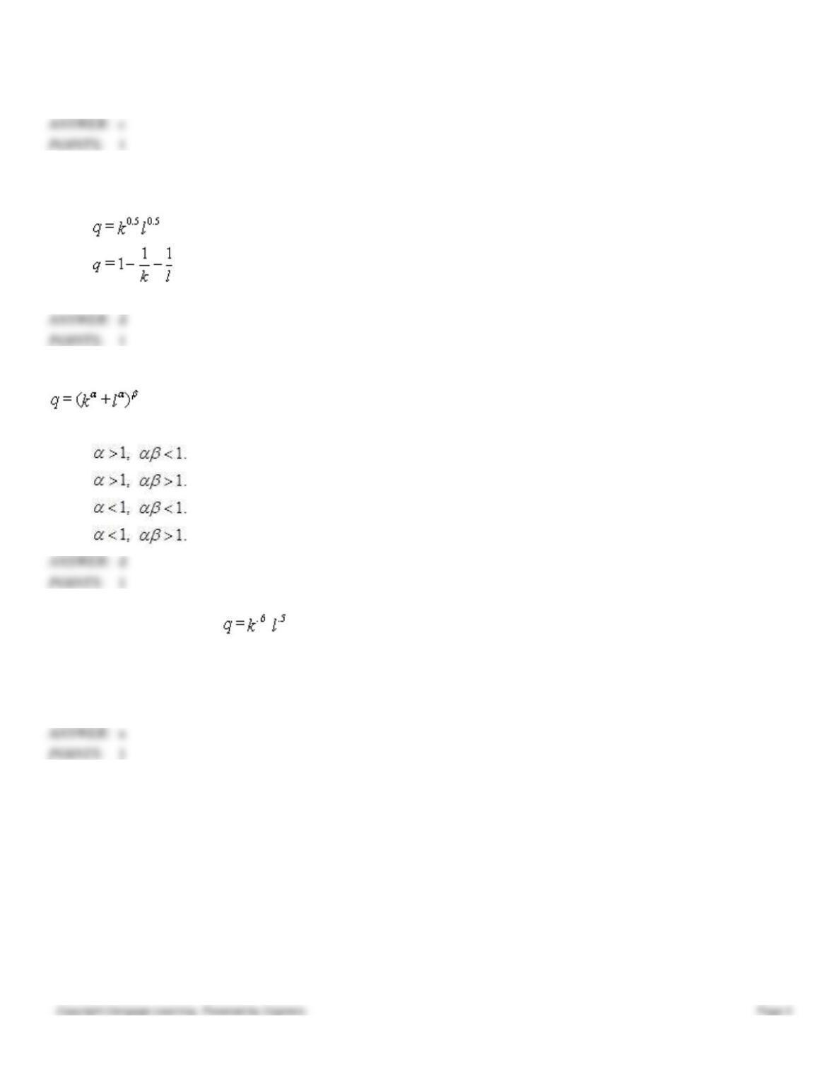
13. Consider the production function
.
For this function to have diminishing marginal productivities and increasing returns to scale, it must be the case that:
a.
b.
c.
d.
14. The production function exhibits:
a.
increasing returns to scale and diminishing marginal products for both k and l.
b.
increasing returns to scale and diminishing marginal product for l only.
c.
increasing returns to scale but no diminishing marginal productivities.
d.
decreasing returns to scale.


