
Introduction to Econometrics, 3e (Stock)
Chapter 9 Assessing Studies Based on Multiple Regression
9.1 Multiple Choice
1) The analysis is externally valid if
A) the statistical inferences about causal effects are valid for the population being studied.
B) the study has passed a double blind refereeing process for a journal.
C) its inferences and conclusions can be generalized from the population and setting studied to other
populations and settings.
D) some committee outside the author’s department has validated the findings.
2) By including another variable in the regression, you will
A) decrease the regression R2 if that variable is important.
B) eliminate the possibility of omitted variable bias from excluding that variable.
C) look at the t–statistic of the coefficient of that variable and include the variable only if the coefficient is
statistically significant at the 1% level.
D) decrease the variance of the estimator of the coefficients of interest.
3) Errors–in–variables bias
A) is present when the probability limit of the OLS estimator is given by
2
11
22
ˆpx
xw
⎯⎯→ + +
.
B) arises when an independent variable is measured imprecisely.
C) arises when the dependent variable is measured imprecisely.
D) always occurs in economics since economic data is never precisely measured.
4) Sample selection bias
A) occurs when a selection process influences the availability of data and that process is related to the
dependent variable.
B) is only important for finite sample results.
C) results in the OLS estimator being biased, although it is still consistent.
D) is more important for nonlinear least squares estimation than for OLS.
5) Simultaneous causality bias
A) is also called sample selection bias.
B) happens in complicated systems of equations called block recursive systems.
C) results in biased estimators if there is heteroskedasticity in the error term.
D) arises in a regression of Y on X when, in addition to the causal link of interest from X to Y, there is a
causal link from Y to X.

6) The reliability of a study using multiple regression analysis depends on all of the following with the
exception of
A) omitted variable bias.
B) errors–in–variables.
C) presence of homoskedasticity in the error term.
D) external validity.
7) A statistical analysis is internally valid if
A) its inferences and conclusions can be generalized from the population and setting studied to other
populations and settings.
B) statistical inference is conducted inside the sample period.
C) the hypothesized parameter value is inside the confidence interval.
D) the statistical inferences about causal effects are valid for the population being studied.
8) The components of internal validity are
A) a large sample, and BLUE property of the estimator.
B) a regression R2 above 0.75 and serially uncorrelated errors.
C) unbiasedness and consistency of the estimator, and desired significance level of hypothesis testing.
D) nonstochastic explanatory variables, and prediction intervals close to the sample mean.
9) A study based on OLS regressions is internally valid if
A) the errors are homoskedastic, and there are no more than two binary variables present among the
regressors.
B) you use a two–sided alternative hypothesis, and standard errors are calculated using the
heteroskedasticity–robust formula.
C) weighted least squares produces similar results, and the t–statistic is normally distributed in large
samples.
D) the OLS estimator is unbiased and consistent, and the standard errors are computed in a way that
makes confidence intervals have the desired confidence level.
10) Panel data estimation can sometimes be used
A) to avoid the problems associated with misspecified functional forms.
B) in case the sum of residuals is not zero.
C) in the case of omitted variable bias when data on the omitted variable is not available.
D) to counter sample selection bias.

11) Misspecification of functional form of the regression function
A) is overcome by adding the squares of all explanatory variables.
B) is more serious in the case of homoskedasticity–only standard error.
C) results in a type of omitted variable bias.
D) requires alternative estimation methods such as maximum likelihood.
12) Errors–in–variables bias
A) is only a problem in small samples.
B) arises from error in the measurement of the independent variable.
C) becomes larger as the variance in the explanatory variable increases relative to the error variance.
D) is particularly severe when the source is an error in the measurement of the dependent variable.
13) A survey of earnings contains an unusually high fraction of individuals who state their weekly
earnings in 100s, such as 300, 400, 500, etc. This is an example of
A) errors–in–variables bias.
B) sample selection bias.
C) simultaneous causality bias.
D) companies that typically bargain with workers in 100s of dollars.
14) In the case of a simple regression, where the independent variable is measured with i.i.d. error,
A)
2
11
22
ˆpX
Xw
⎯⎯→ +
B)
2
122
1
ˆpX
Xw
⎯⎯→ +
.
C)
2
11
22
ˆpw
Xw
⎯⎯→ +
.
D)
2
11
22
ˆpX
Xw
⎯⎯→ + +
.
15) In the case of errors–in–variables bias,
A) maximum likelihood estimation must be used.
B) the OLS estimator is consistent if the variance in the unobservable variable is relatively large compared
to variance in the measurement error.
C) the OLS estimator is consistent, but no longer unbiased in small samples.
D) binary variables should not be used as independent variables.

16) Sample selection bias occurs when
A) the choice between two samples is made by the researcher.
B) data are collected from a population by simple random sampling.
C) samples are chosen to be small rather than large.
D) the availability of the data is influenced by a selection process that is related to the value of the
dependent variable.
17) Simultaneous causality
A) means you must run a second regression of X on Y.
B) leads to correlation between the regressor and the error term.
C) means that a third variable affects both Y and X.
D) cannot be established since regression analysis only detects correlation between variables.
18) Correlation of the regression error across observations
A) results in incorrect OLS standard errors.
B) makes the OLS estimator inconsistent, but not unbiased.
C) results in correct OLS standard errors if heteroskedasticity–robust standard errors are used.
D) is not a problem in cross–sections since the data can always be “reshuffled.”
19) Applying the analysis from the California test scores to another U.S. state is an example of looking for
A) simultaneous causality bias.
B) external validity.
C) sample selection bias.
D) internal validity.
20) Comparing the California test scores to test scores in Massachusetts is appropriate for external
validity if
A) Massachusetts also allowed beach walking to be an appropriate P.E. activity.
B) the two income distributions were very similar.
C) the student–to–teacher ratio did not differ by more than five on average.
D) the institutional settings in California and Massachusetts, such as organization in classroom
instruction and curriculum, were similar in the two states.
21) The guidelines for whether or not to include an additional variable include all of the following, with
the exception of
A) providing “full disclosure” representative tabulations of the results.
B) testing whether additional questionable variables have nonzero coefficients.
C) determining whether it can be measured in the population of interest.
D) being specific about the coefficient or coefficients of interest.

22) Possible solutions to omitted variable bias, when the omitted variable is not observed, include the
following with the exception of
A) panel data estimation.
B) nonlinear least squares estimation.
C) use of instrumental variables regressions.
D) use of randomized controlled experiments.
23) A possible solution to errors–in–variables bias is to
A) use log–log specifications.
B) choose different functional forms.
C) use the square root of that variable since the error becomes smaller.
D) mitigate the problem through instrumental variables regression.
24) You try to explain the number of IBM shares traded in the stock market per day in 2005. As an
independent variable you choose the closing price of the share. This is an example of
A) simultaneous causality.
B) invalid inference due to a small sample size.
C) sample selection bias since you should analyze more than one stock.
D) a situation where homoskedasticity–only standard errors should be used since you only analyze one
company.
25) In the case of errors–in–variables bias, the precise size and direction of the bias depend
on
A) the sample size in general.
B) the correlation between the measured variable and the measurement error.
C) the size of the regression R2.
D) whether the good in question is price elastic.
26) The question of reliability/unreliability of a multiple regression depends on
A) internal but not external validity
B) the quality of your statistical software package
C) internal and external validity
D) external but not internal validity
27) A statistical analysis is internally valid if
A) all t–statistics are greater than |1.96|
B) the regression R2 > 0.05
C) the population is small, say less than 2,000, and can be observed
D) the statistical inferences about causal effects are valid for the population studied

28) A definition of internal validity is
A) the estimator of the causal effect being unbiased and consistent
B) the estimator of the causal effect being efficient
C) inferences and conclusions being generalized from the population to other populations
D) OLS estimation being available in your statistical package
29) Threats to in internal validity lead to
A) perfect multicollinearity
B) the inability to transfer data sets into your statistical package
C) failures of one or more of the least squares assumptions
D) a false generalization to the population of interest
30) The true causal effect might not be the same in the population studied and the population of interest
because
A) of differences in characteristics of the population
B) of geographical differences
C) the study is out of date
D) all of the above

9.2 Essays and Longer Questions
1) Until about 10 years ago, most studies in labor economics found a small but significant negative
relationship between minimum wages and employment for teenagers. Two labor economists challenged
this perceived wisdom with a publication in 1992 by comparing employment changes of fast–food
restaurants in Texas, before and after a federal minimum wage increase.
(a) Explain how you would obtain external validity in this field of study.
(b) List the various threats to external validity and suggest how to address them in this case.

8
2) Your textbook used the California Standardized Testing and Reporting (STAR) data set on test student
performance in Chapters 4–7. One justification for putting second to twelfth graders through such an
exercise once a year is to make schools more accountable. The hope is that schools with low scores will
improve the following year and in the future. To test for the presence of such an effect, you collect data
from 1,000 L.A. County schools for grade 4 scores in 1998 and 1999, both for reading (Read) and
mathematics (Maths). Both are on a scale from zero to one hundred. The regression results are as follows
(homoskedasticity–only standard errors in parentheses):
= 6.967 + 0.919 , R2 = 0.825, SER = 7.818
(0.542) (0.013)
= 4.131 + 0.943, = R2 = 0.887, SER = 6.416
(0.409) (0.011)
(a) Interpret the results and indicate whether or not the coefficients are significantly different from zero.
Do the coefficients have the expected sign and magnitude?
(b) Discuss various threats to internal and external validity, and try to assess whether or not these are
likely to be present in your study.
(c) Changing the estimation method to allow for heteroskedasticity–robust standard errors produces four
new standard errors: (0.539), (0.015), (0.452), and (0.015) in the order of appearance in the two equations
above. Given these numbers, do any of your statements in (b) change? Do you think that the coefficients
themselves changed?
(d) If reading and maths scores were the same in 1999 as in 1998, on average, what coefficients would you
expect for the intercept and the slope? How would you test for the restrictions?
(e) The appropriate F–statistic in (d) is 138.27 for the maths scores, and 104.85 for the reading scores.
Comparing these values to the critical values in the F table, can you reject the null hypothesis in each
case?
(f) Your professor tells you that the analysis reminds her of “Galton’s Fallacy.” Sir Francis Galton
regressed the height of children on the average height of their parents. He found a positive intercept and
a slope between zero and one. Being concerned about the height of the English aristocracy, he interpreted
the results as “regression to mediocrity” (hence the name regression). Do you see the parallel?


10
3) Keynes postulated that the marginal propensity to consume (MPC = ) is between zero and one.
He also hypothesized that the average propensity to consume (APC = ) would fall as personal
disposable income increased.
(a) Specify a linear consumption function. Show that the assumption of a falling APC implies the
presence of a positive intercept.
(b) Using annual per capita data, estimation of the consumption function for the United States results in
the following output for the years 1929–1938:
= 981.35 + 0.735 , R2 = 0.98, SER= 50.65
(158.65) (0.038)
Can you reject the null hypothesis that the slope is less than one? Greater than zero? Test the hypothesis
that the intercept is zero. Should you be concerned about the sample size when conducting these tests?
What other threats to internal validity may be present here?
(c) Given the GDP identity for a closed economy,
,
t t t t
Y C I G + +
show why economists saw important policy implications in finding an APC that would decrease over
time.
(d) Simon Kuznets, who won the Nobel Prize in economics, collected data on consumption expenditures
and national income from 1869 to 1938 and found, using overlapping period averages, that the APC was
relatively constant over this period. To reconcile this finding with the regression results, Milton
Friedman, who also won the Nobel Prize, formulated the “permanent income” hypothesis. In essence,
Friedman hypothesized that both actual consumption and income are measured with error,
ttt
C C v=+
and
,
ttt
Y Y w=+
where
t
C
and
t
Y
were called “permanent” consumption and income, respectively, and
t
v
and
t
w
, the
two measurement errors, were labeled transitory consumption and income. Friedman hypothesized that
the transitory components were purely random error terms, uncorrelated with the permanent parts.
Let permanent consumption and income be related as follows:
,t pd t t
C k Y u= +
so that the APC and MPC are the same and constant over time. Furthermore, let both transitory and
permanent income be independent of the error term. Show that by regressing actual consumption on
actual income, the MPC will be downward biased, and the intercept will be greater than zero, even in
large samples (to simplify the analysis, assume that permanent income and all of the errors are i.i.d. and
mutually independent).
4) The Phillips curve is a relationship in macroeconomics between the inflation rate (inf) and the
unemployment rate (ur). Estimating the Phillips curve using quarterly data for the United States from
1962:I to 1995:IV, you find
= 4.08 + 0.118 urt, R2 = 0.003, SER = 3.148
(1.11) (0.176)
(a) Explain why, at first glance, this is a surprising result.
(b) Do you think that there is omitted variable bias in the regression?
(c) What other threats to internal validity may be present?
(d) If you could find a proper specification for the Phillips curve using United States data, what external
validity criteria would you suggest?
12
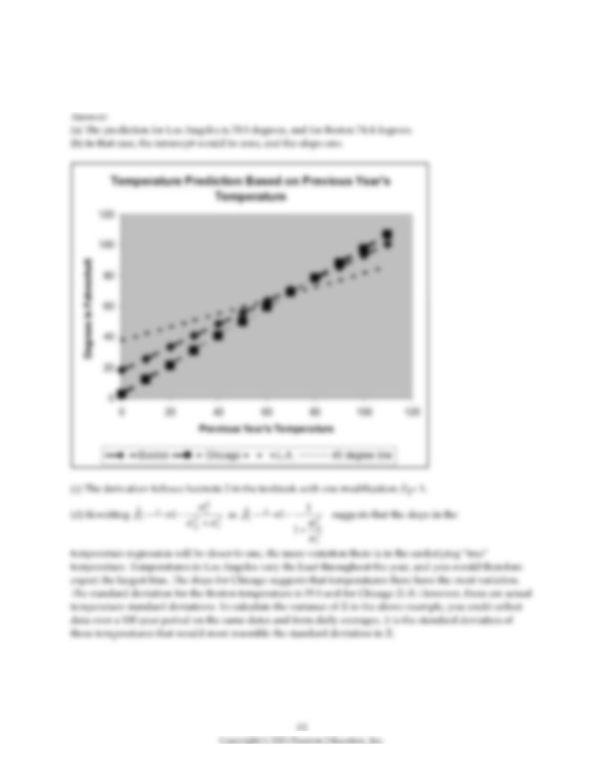
5) You have decided to analyze the year–to–year variation in temperature data. Specifically you want to
use this year’s temperature to predict next year’s temperature for certain cities. As a result, you collect the
daily high temperature (Temp) for 100 randomly selected days in a given year for three United States
cities: Boston, Chicago, and Los Angeles. You then repeat the exercise for the following year. The
regression results are as follows (heteroskedasticity–robust standard errors in parentheses):
= 18.19 + 0.75 ×; R2 = 0.62, SER = 12.33
(6.46) (0.10)
= 2.47 + 0.95 ×; R2 = 0.93, SER = 5.85
(3.98) (0.05)
= 37.54 + 0.44 ×; R2 = 0.18, SER = 7.17
(15.33) (0.22)
(a) What is the prediction of the above regression for Los Angeles if the temperature in the previous year
was 75 degrees? What would be the prediction for Boston?
(b) Assume that the previous year’s temperature gives accurate predictions, on average, for this year’s
temperature. What values would you expect in this case for the intercept and slope? Sketch how each of
the above regressions behaves compared to this line.
(c) After reflecting on the results a bit, you consider the following explanation for the above results. Daily
high temperatures on any given date are measured with error in the following sense: for any given day in
any of the three cities, say January 28, there is a true underlying seasonal temperature (X), but each year
there are different temporary weather patterns (v, w) which result in a temperature different from X.
For the two years in your data set, the situation can be described as follows:
= X + vt and = X + wt
Subtracting from , you get = + wt – vt. Hence the population parameter for the intercept
and slope are zero and one, as expected. Show that the OLS estimator for the slope is inconsistent, where
2
122
ˆ1
p
X
⎯⎯→ − +
(d) Use the formula above to explain the differences in the results for the three cities. Is your
mathematical explanation intuitively plausible?

14
6) A study of United States and Canadian labor markets shows that aggregate unemployment rates
between the two countries behaved very similarly from 1920 to 1982, when a two percentage point gap
opened between the two countries, which has persisted over the last 20 years. To study the causes of this
phenomenon, you specify a regression of Canadian unemployment rates on demographic variables,
aggregate demand variables, and labor market characteristics.
(a) Assume that your analysis is internally valid. What would make it externally valid?
(b) If one of the determinants of Canadian unemployment is aggregate United States economic activity
(or perhaps shocks to it), what variable would you suggest as its replacement if you did a similar study
for the United States?
(c) Certain Canadian geographical areas, such as the prairies and British Columbia, seem particularly
sensitive to commodity price shocks (Edmonton’s NHL team is called the Edmonton Oilers). Having
collected provincial data, you establish a relationship between provincial unemployment rates and
commodity price changes (shocks). How would you address external validity now?
7) Several authors have tried to measure the “persistence” in U.S state unemployment rates by running
the following regression:
, 0 1 , ,i t i t k i t
ur ur z
−
= + +
where ur is the state unemployment rate, i is the index for the i–th state, t indicates a time period, and
typically k ≥ 10.
(a) Explain why finding a slope estimate of one and an intercept of zero is typically interpreted as
evidence of “persistence.”
(b) You collect data on the 48 contiguous U.S. states’ unemployment rates and find the following
estimates:
,1995
ˆi
ur
= 2.25 + 0.60 ×
,1970i
ur
; R2 = 0.40, SER = 0.90
(0.61) (0.13)
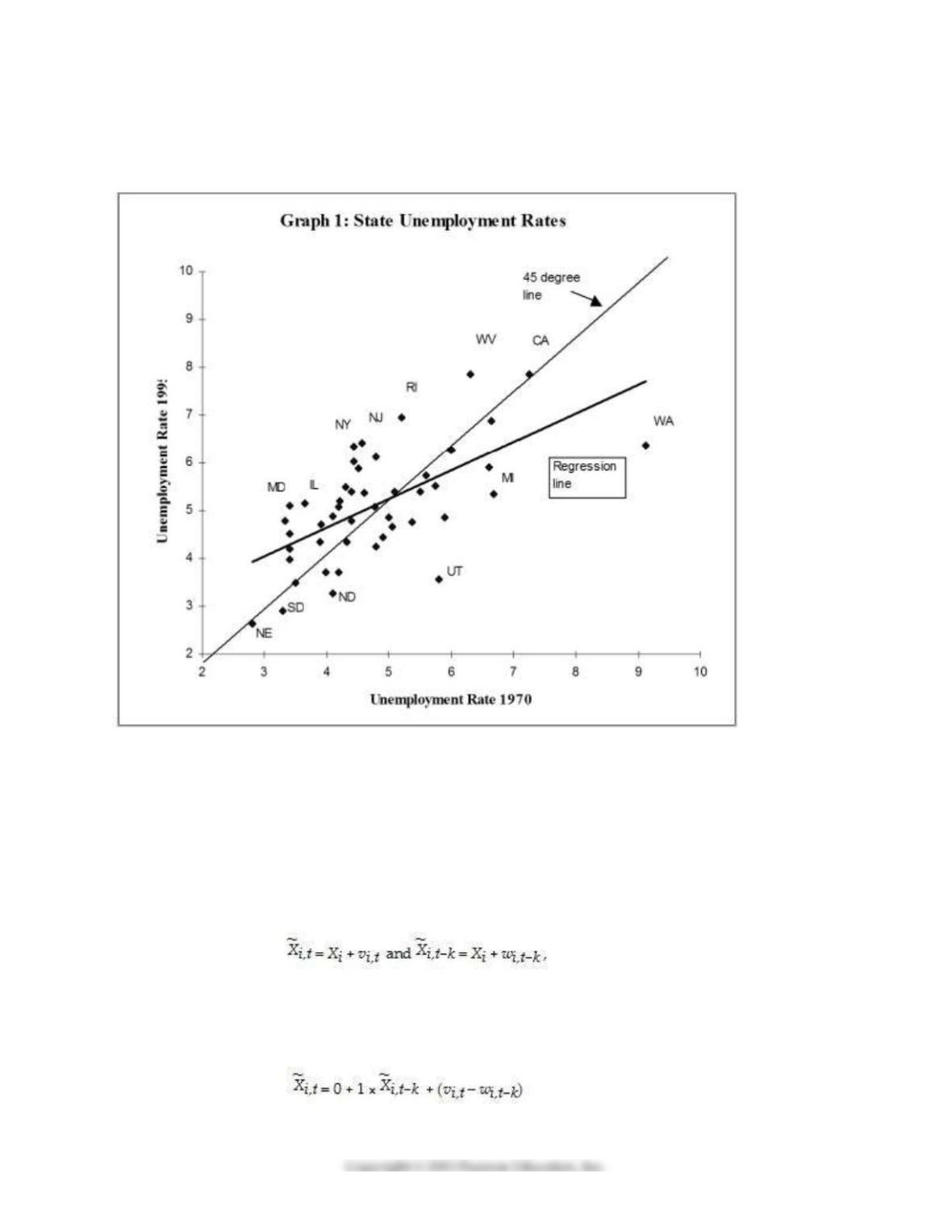
15
Interpret the regression results.
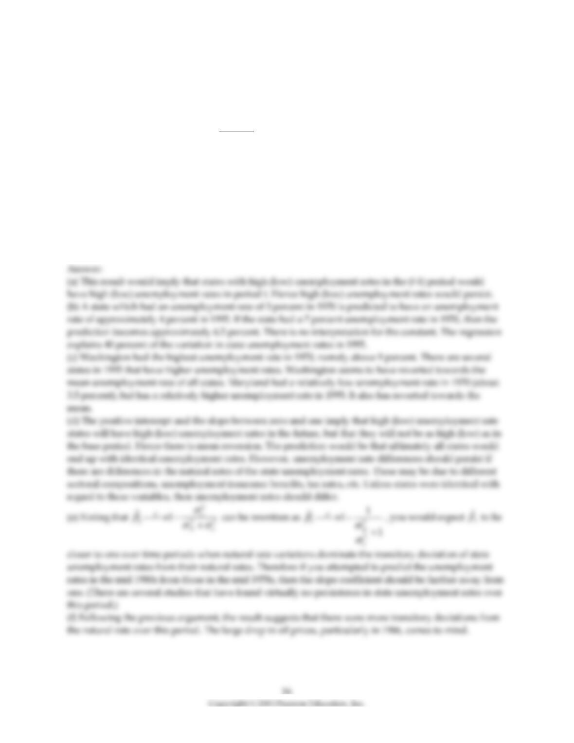
(c) Analyzing the accompanying figure, and interpret the observation for Maryland and for Washington.
Do you find evidence of persistence? How would you test for it?
(d) One of your peers points out that this result makes little sense, since it implies that eventually all
states would have identical unemployment rates. Explain the argument.
(e) Imagine that state unemployment rates were determined by their natural rates and some transitory
shock. The natural rates themselves may be functions of the unemployment insurance benefits of the
state, unionization rates of its labor force, demographics, sectoral composition, etc. The transitory
components may include state–specific shocks to its terms of trade such as raw material movements and
demand shocks from the other states. You specify the i–th state unemployment rate accordingly as
follows for the two periods when you observe it,
so that actual unemployment rates are measured with error. You have also assumed that the natural rate
is the same for both periods. Subtracting the second period from the first then results in the following
population regression function:
It is not too hard to show that estimation of the observed unemployment rate in period t on the
unemployment rate in period (t–k) by OLS results in an estimator for the slope coefficient that is biased
towards zero. The formula is
2
122
ˆ1
p
X
⎯⎯→ − +
.
Using this insight, explain over which periods you would expect the slope to be closer to one, and over
which period it should be closer to zero.
(f) Estimating the same regression for a different time period results in
,1995
ˆi
ur
= 3.19 + 0.27 ×
,1985
ˆi
ur
; R2 = 0.21, SER = 1.03
(0.56) (0.07)
If your above analysis is correct, what are the implications for this time period?

17
8) Sir Francis Galton (1822–1911), an anthropologist and cousin of Charles Darwin, created the term
regression. In his article “Regression towards Mediocrity in Hereditary Stature,” Galton compared the
height of children to that of their parents, using a sample of 930 adult children and 205 couples. In
essence he found that tall (short) parents will have tall (short) offspring, but that the children will not be
quite as tall (short) as their parents, on average. Hence there is regression towards the mean, or as Galton
referred to it, mediocrity. This result is obviously a fallacy if you attempted to infer behavior over time
since, if true, the variance of height in humans would shrink over generations. This is not the case.
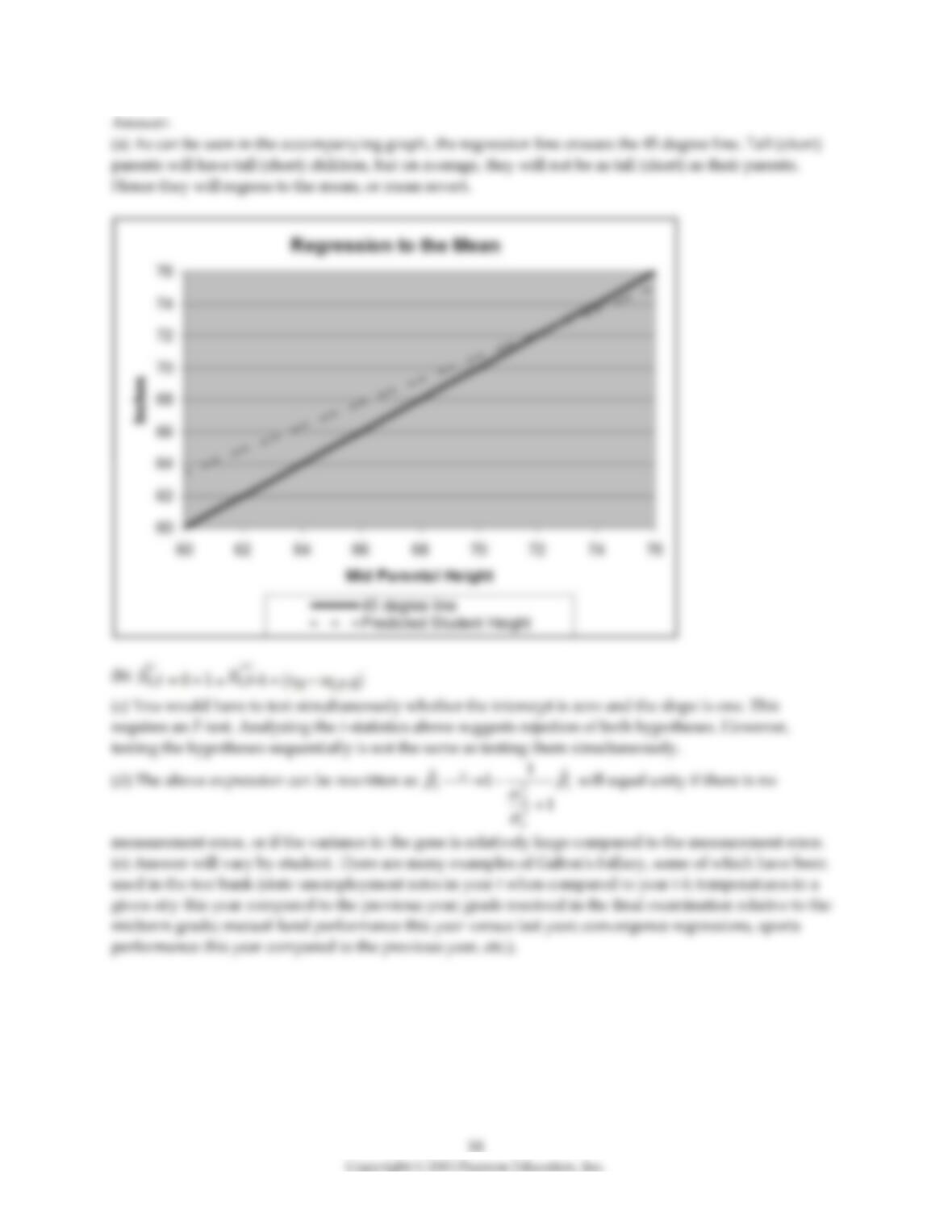
(a) To research this result, you collect data from 110 college students and estimate the following
relationship:
= 19.6 + 0.73 × Midparh, R2 = 0.45, SER = 2.0
(7.2) (0.10)
where Studenth is the height of students in inches and Midparh is the average of the parental heights.
Values in parentheses are heteroskedasticity–robust standard errors. Sketching this regression line
together with the 45 degree line, explain why the above results suggest “regression to the mean” or “mean
reversion.”
(b) Researching the medical literature, you find that height depends, to a large extent, on one gene
(“phog”) and on environmental influences. Let us assume that parents and offspring have the same
invariant (over time) gene and that actual height is therefore measured with error in the following sense,
where
X
is measured height, X is the height given through the gene, v and w are environmental
influences, and the subscripts o and p stand for offspring and parents, respectively. Let the
environmental influences be independent from each other and from the gene.
Subtracting the measured height of offspring from the height of parents, what sort of population
regression function do you expect?
(c) How would you test for the two restrictions implicit in the population regression function in (b)? Can
you tell from the results in (a) whether or not the restrictions hold?
(d) Proceeding in a similar way to the proof in your textbook, you can show that
2
122
ˆ1
p
X
⎯⎯→ − +
for the situation in (b). Discuss under what conditions you will find a slope closer to one for the height
comparison. Under what conditions will you find a slope closer to zero?
(e) Can you think of other examples where Galton’s Fallacy might apply?

19
9) Macroeconomists who study the determinants of per capita income (the “wealth of nations”) have been
particularly interested in finding evidence on conditional convergence in the countries of the world.
Finding such a result would imply that all countries would end up with the same per capita income once
other variables such as saving and population growth rates, education, government policies, etc., took on
the same value. Unconditional convergence, on the other hand, does not control for these additional
variables.
(a) The results of the regression for 104 countries was as follows,
= 0.019 – 0.0006 × RelProd60, R2= 0.00007, SER = 0.016
(0.004) (0.0073),
where g6090 is the average annual growth rate of GDP per worker for the 1960–1990 sample period, and
RelProd60 is GDP per worker relative to the United States in 1960.
For the 24 OECD countries in the sample, the output is
= 0.048 – 0.0404 RelProd60, R2 = 0.82, SER = 0.0046
(0.004) (0.0063)
Interpret the results and point out the difference with regard to unconditional convergence.
(b) The “beta–convergence” regressions in (a) are of the following type,
= β0 + β0 ln Yi,0 + ui,t,
where
△
t ln Yi,t = ln Yi,0 – ln Yi,0, and t and o refer to two time periods, i is the i–th country.
Explain why a significantly negative slope implies convergence (hence the name).
(c) The equation in (b) can be rewritten without any change in information as (ignoring the division by T)
ln Yt = β0 + γ1 ln Y0 + ut
In this form, how would you test for unconditional convergence? What would be the implication for
convergence if the slope coefficient were one?
(d) Let’s write the equation in (c) as follows:
and assume that the “~” variables contain measurement errors of the following type,