Chapter 8/Application: The Costs of Taxation ❖ 61
42. Taxes on labor have the effect of encouraging
a.
workers to work more hours.
b.
the elderly to postpone retirement.
c.
second earners within a family to take a job.
d.
unscrupulous people to take part in the underground economy.
43. Concerning the labor market and taxes on labor, economists disagree about
a.
the size of the tax on labor.
b.
the size of the deadweight loss of the tax on labor.
c.
whether or not a tax on labor places a wedge between the wage that firms pay and the wage that
workers receive.
d.
All of the above are correct.
44. The Social Security tax is a tax on
a.
capital.
b.
labor.
c.
consumption expenditures.
d.
earnings during retirement.
45. If the labor supply curve is nearly vertical, a tax on labor
a.
has a large deadweight loss.
b.
raises a small amount of tax revenue.
c.
has little impact on the amount of work that workers are willing to do.
d.
results in a large tax burden on the firms that hire labor.
46. If the labor supply curve is very elastic, a tax on labor
a.
has a large deadweight loss.
b.
raises enough tax revenue to offset the loss in welfare.
c.
has a relatively small impact on the number of hours that workers choose to work.
d.
results in a large tax burden on the firms that hire labor.
47. The marginal tax rate on labor income for many workers in the United States is almost
a.
30 percent.
b.
40 percent.
c.
50 percent.
d.
65 percent.
62 ❖ Chapter 8/Application: The Costs of Taxation
48. The more freedom young mothers have to work outside the home, the
a.
more elastic the supply of labor will be.
b.
less elastic the supply of labor will be.
c.
more vertical the labor supply curve will be.
d.
smaller is the decrease in employment that will result from a tax on labor.
49. The less freedom people are given to choose the date of their retirement, the
a.
more elastic is the supply of labor.
b.
less elastic is the supply of labor.
c.
flatter is the labor supply curve.
d.
smaller is the decrease in employment that will result from a tax on labor.
50. Taxes on labor encourage all of the following except
a.
older workers to take early retirement from the labor force.
b.
mothers to stay at home rather than work in the labor force.
c.
workers to work overtime.
d.
people to be paid “under the table.”
51. Taxes on labor encourage which of the following?
a.
labor demand to be more inelastic
b.
mothers to stay at home rather than work in the labor force
c.
workers to work overtime
d.
fathers to take on second jobs
52. As more people become self-employed, which allows them to determine how many hours they work per week,
we would expect the deadweight loss from the Social Security tax to
a.
increase, and the revenue generated from the tax to increase.
b.
increase, and the revenue generated from the tax to decrease.
c.
decrease, and the revenue generated from the tax to increase.
d.
decrease, and the revenue generated from the tax to decrease.
53. Which of the following is not correct?
a.
Economists who argue that labor taxes are highly distorting believe that labor supply is fairly
elastic.
b.
Economists who argue that labor taxes are not highly distorting believe that labor supply is fairly
inelastic.
c.
Economists who argue that labor supply is fairly inelastic cite elderly workers who adjust the date
they retire as an example.
d.
Economists who argue that labor supply is fairly elastic cite workers who adjust the hours of
overtime that they work as an example.
Chapter 8/Application: The Costs of Taxation ❖ 63
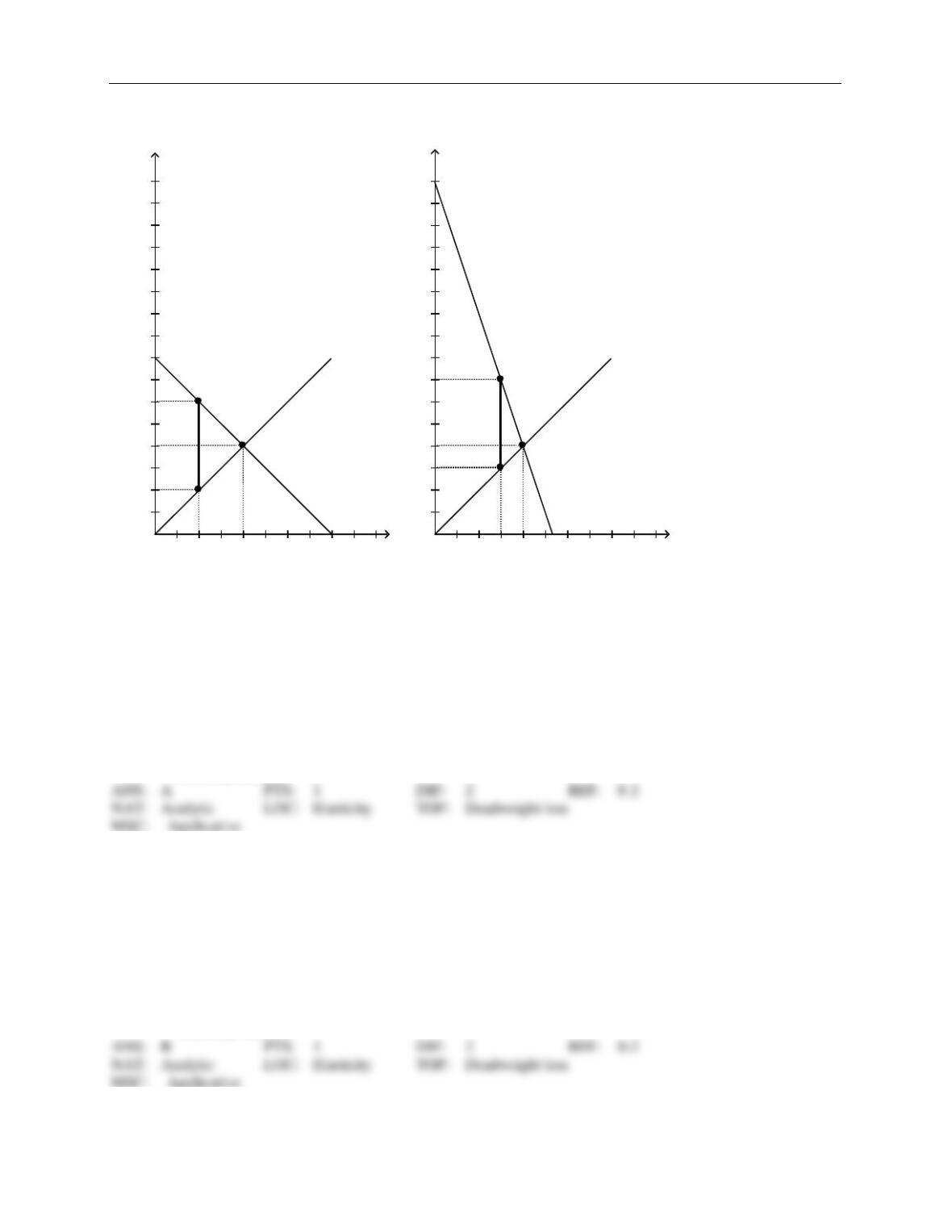
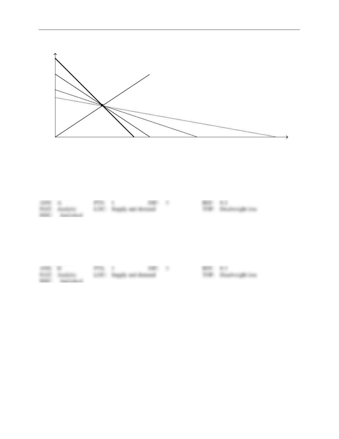
Figure 8-13
Demand
Supply
Panel (a)
1 2 3 4 5 6 7 8 Quantity
1
2
3
4
5
6
7
8
9
10
11
12
13
14
15
16
Price
Demand
Supply
Panel (b)
1 2 3 4 5 6 7 8 Quantity
1
2
3
4
5
6
7
8
9
10
11
12
13
14
15
16
Price
54. Refer to Figure 8-13. Panel (a) and Panel (b) each illustrate a $4 tax placed on a market. In comparison to
Panel (a), Panel (b) illustrates which of the following statements?
a.
When demand is relatively inelastic, the deadweight loss of a tax is smaller than when demand is
relatively elastic.
b.
When demand is relatively elastic, the deadweight loss of a tax is larger than when demand is
relatively inelastic.
c.
When supply is relatively inelastic, the deadweight loss of a tax is smaller than when supply is
relatively elastic.
d.
When supply is relatively elastic, the deadweight loss of a tax is larger than when supply is
relatively inelastic.
55. Refer to Figure 8-13. Panel (a) and Panel (b) each illustrate a $4 tax placed on a market. In comparison to
Panel (b), Panel (a) illustrates which of the following statements?
a.
When demand is relatively inelastic, the deadweight loss of a tax is smaller than when demand is
relatively elastic.
b.
When demand is relatively elastic, the deadweight loss of a tax is larger than when demand is
relatively inelastic.
c.
When supply is relatively inelastic, the deadweight loss of a tax is smaller than when supply is
relatively elastic.
d.
When supply is relatively elastic, the deadweight loss of a tax is larger than when supply is
relatively inelastic.
64 ❖ Chapter 8/Application: The Costs of Taxation
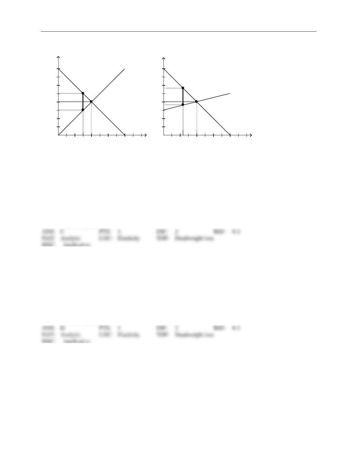
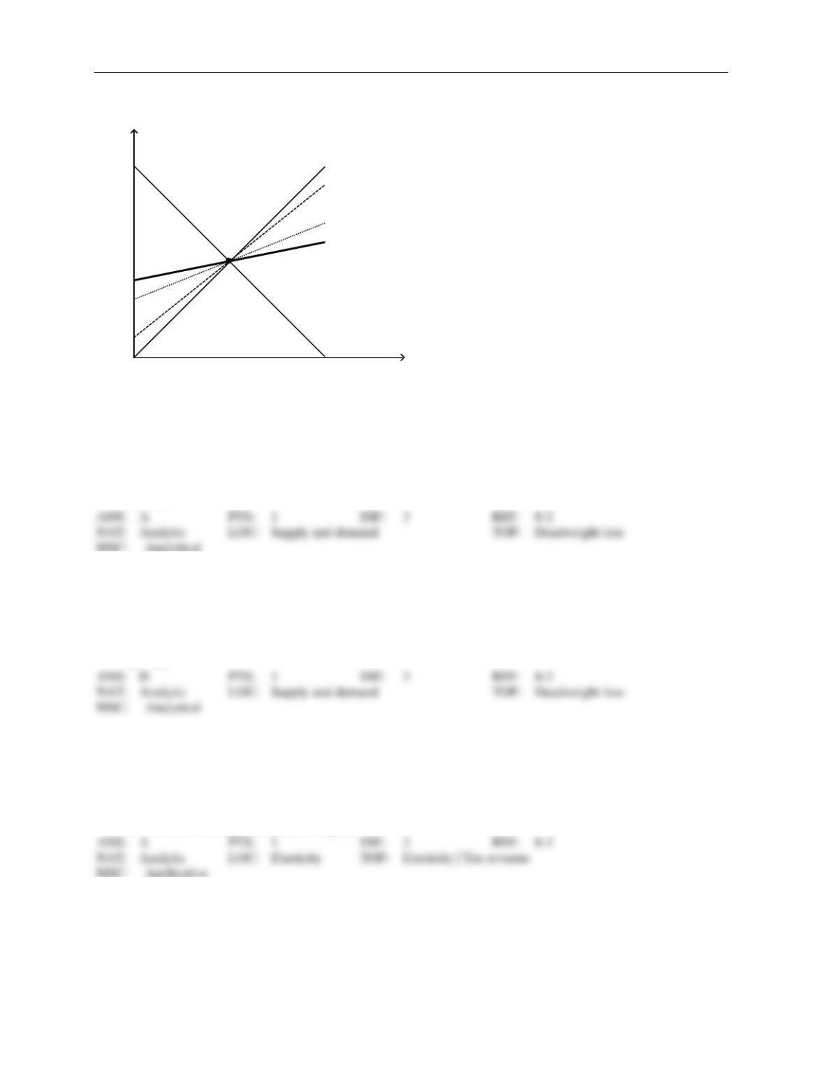
Figure 8-14
Demand
Supply
Panel (a)
1 2 3 4 5 6 7 8 Quantity
1
2
3
4
5
6
7
8
Price
Demand
Panel (b)
Supply
1 2 3 4 5 6 7 8 Quantity
1
2
3
4
5
6
7
8
Price
56. Refer to Figure 8-14. Panel (a) and Panel (b) each illustrate a $2 tax placed on a market. In comparison to
Panel (b), Panel (a) illustrates which of the following statements?
a.
When demand is relatively inelastic, the deadweight loss of a tax is smaller than when demand is
relatively elastic.
b.
When demand is relatively elastic, the deadweight loss of a tax is larger than when demand is
relatively inelastic.
c.
When supply is relatively inelastic, the deadweight loss of a tax is smaller than when supply is
relatively elastic.
d.
When supply is relatively elastic, the deadweight loss of a tax is larger than when supply is
relatively inelastic.
57. Refer to Figure 8-14. Panel (a) and Panel (b) each illustrate a $2 tax placed on a market. In comparison to
Panel (a), Panel (b) illustrates which of the following statements?
a.
When demand is relatively inelastic, the deadweight loss of a tax is smaller than when demand is
relatively elastic.
b.
When demand is relatively elastic, the deadweight loss of a tax is larger than when demand is
relatively inelastic.
c.
When supply is relatively inelastic, the deadweight loss of a tax is smaller than when supply is
relatively elastic.
d.
When supply is relatively elastic, the deadweight loss of a tax is larger than when supply is
relatively inelastic.
Chapter 8/Application: The Costs of Taxation ❖ 65
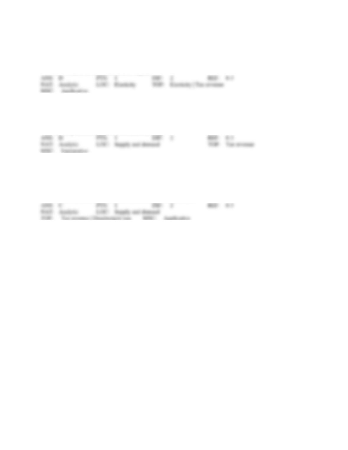
Figure 8-15
D1 D2
S
D3 D4
Quantity
Price
58. Refer to Figure 8-15. Suppose the government imposes a $1 tax in each of the four markets represented by
demand curves D1, D2, D3, and D4. The deadweight will be the smallest in the market represented by
a.
D1.
b.
D2.
c.
D3.
d.
D4.
59. Refer to Figure 8-15. Suppose the government imposes a $1 tax in each of the four markets represented by
demand curves D1, D2, D3, and D4. The deadweight will be the largest in the market represented by
a.
D1.
b.
D2.
c.
D3.
d.
D4.
66 ❖ Chapter 8/Application: The Costs of Taxation
Figure 8-16
D
S1
S2
S3
S4
Quantity
Price
60. Refer to Figure 8-16. Suppose the government imposes a $1 tax in each of the four markets represented by
supply curves S1, S2, S3, and S4. The deadweight will be the smallest in the market represented by
a.
S1.
b.
S2.
c.
S3.
d.
S4.
61. Refer to Figure 8-16. Suppose the government imposes a $1 tax in each of the four markets represented by
supply curves S1, S2, S3, and S4. The deadweight will be the largest in the market represented by
a.
S1.
b.
S2.
c.
S3.
d.
S4.
DEADWEIGHT LOSS AND TAX REVENUE AS TAXES VARY
1. A decrease in the size of a tax is most likely to increase tax revenue in a market with
a.
elastic demand and elastic supply.
b.
elastic demand and inelastic supply.
c.
inelastic demand and elastic supply.
d.
inelastic demand and inelastic supply.
Chapter 8/Application: The Costs of Taxation ❖ 67
2. An increase in the size of a tax is most likely to increase tax revenue in a market with
a.
elastic demand and elastic supply.
b.
elastic demand and inelastic supply.
c.
inelastic demand and elastic supply.
d.
inelastic demand and inelastic supply.
3. If the size of a tax increases, tax revenue
a.
increases.
b.
decreases.
c.
remains the same.
d.
may increase, decrease, or remain the same.
4. Suppose the tax on liquor is increased so that the tax goes from being a “medium” tax to being a “large” tax.
As a result, it is likely that
a.
tax revenue increases, and the deadweight loss increases.
b.
tax revenue increases, and the deadweight loss decreases.
c.
tax revenue decreases, and the deadweight loss increases.
d.
tax revenue decreases, and the deadweight loss decreases.
68 ❖ Chapter 8/Application: The Costs of Taxation
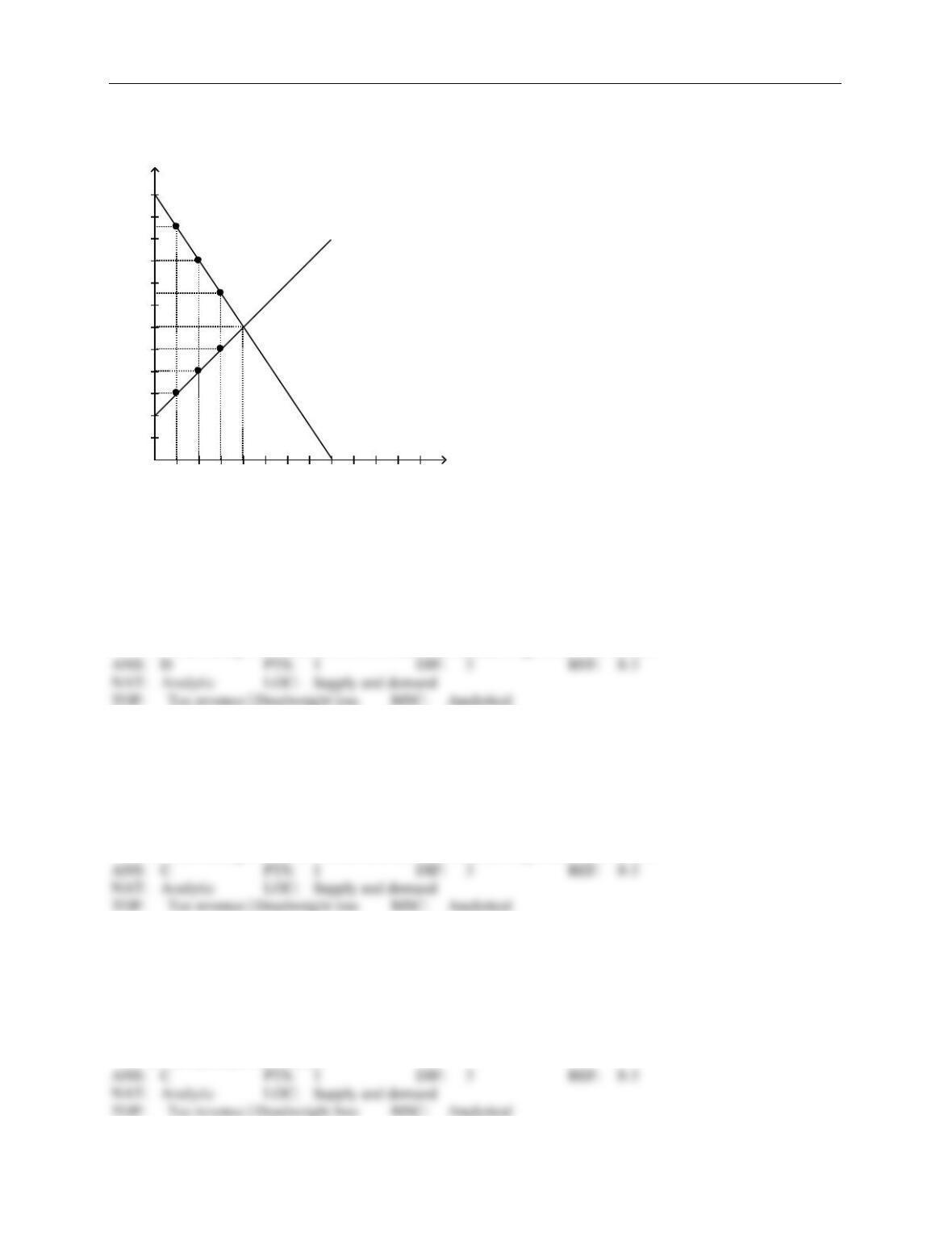
Figure 8-17
The vertical distance between points A and B represents the original tax.
S
D
A
B
D
C
G
F
0.5 1 1.5 2 2.5 3 3.5 4 4.5 5 Quantity
1
2
3
4
5
6
7
8
9
10
11
12
Price
5. Refer to Figure 8-17. If the government changed the per-unit tax from $5.00 to $2.50, then the price paid by
buyers would be $7.50, the price received by sellers would be $5, and the quantity sold in the market would be
1.5 units. Compared to the original tax rate, this lower tax rate would
a.
increase government revenue and increase the deadweight loss from the tax.
b.
increase government revenue and decrease the deadweight loss from the tax.
c.
decrease government revenue and increase the deadweight loss from the tax.
d.
decrease government revenue and decrease the deadweight loss from the tax.
6. Refer to Figure 8-17. If the government changed the per-unit tax from $5.00 to $7.50, then the price paid by
buyers would be $10.50, the price received by sellers would be $3, and the quantity sold in the market would
be 0.5 units. Compared to the original tax rate, this higher tax rate would
a.
increase government revenue and increase the deadweight loss from the tax.
b.
increase government revenue and decrease the deadweight loss from the tax.
c.
decrease government revenue and increase the deadweight loss from the tax.
d.
decrease government revenue and decrease the deadweight loss from the tax.
7. Refer to Figure 8-17. The original tax can be represented by the vertical distance AB. Suppose the govern-
ment is deciding whether to lower the tax to CD or raise it to FG. Which of the following statements is cor-
rect?
a.
Compared to the original tax, the larger tax will decrease both tax revenue and deadweight loss.
b.
Compared to the original tax, the smaller tax will increase both tax revenue and deadweight loss.
c.
Compared to the original tax, the larger tax will decrease tax revenue and increase deadweight loss.
d.
Both a and b are correct.

Chapter 8/Application: The Costs of Taxation ❖ 69
8. Refer to Figure 8-17. The original tax can be represented by the vertical distance AB. Suppose the govern-
ment is deciding whether to lower the tax to CD or raise it to FG. Which of the following statements is not
correct?
a.
Compared to the original tax, the larger tax will increase tax revenue.
b.
Compared to the original tax, the smaller tax will decrease deadweight loss.
c.
Compared to the original tax, the smaller tax will decrease tax revenue.
d.
Compared to the original tax, the larger tax will increase deadweight loss.
9. As the tax on a good increases from $1 per unit to $2 per unit to $3 per unit and so on, the
a.
tax revenue increases at first, but it eventually peaks and then decreases.
b.
deadweight loss increases at first, but it eventually peaks and then decreases.
c.
tax revenue always increases, and the deadweight loss always increases.
d.
tax revenue always decreases, and the deadweight loss always increases.
10. Which of the following ideas is the most plausible?
a.
Tax revenue is more likely to increase when a low tax rate is increased than when a high tax rate is
increased.
b.
Tax revenue is less likely to increase when a low tax rate is increased than when a high tax rate is
increased.
c.
Tax revenue is likely to increase by the same amount when a low tax rate is increased and when a
high tax rate is increased.
d.
Decreasing a tax rate can never increase tax revenue.
11. Which of the following statements is true for markets in which the demand curve slopes downward and the
supply curve slopes upward?
a.
As the size of the tax increases, tax revenue continually rises and deadweight loss continually falls.
b.
As the size of the tax increases, tax revenue and deadweight loss rise initially, but both eventually
begin to fall.
c.
As the size of the tax increases, tax revenue rises initially, but it eventually begins to fall;
deadweight loss continually rises.
d.
As the size of the tax increases, tax revenue rises initially, but it eventually begins to fall;
deadweight loss falls initially, but eventually it begins to rise.
12. In which of the following cases is it most likely that an increase in the size of a tax will decrease tax revenue?
a.
The price elasticity of demand is small, and the price elasticity of supply is large.
b.
The price elasticity of demand is large, and the price elasticity of supply is small.
c.
The price elasticity of demand and the price elasticity of supply are both small.
d.
The price elasticity of demand and the price elasticity of supply are both large.

70 ❖ Chapter 8/Application: The Costs of Taxation
13. Which of the following statements correctly describes the relationship between the size of the deadweight loss
and the amount of tax revenue as the size of a tax increases from a small tax to a medium tax and finally to a
large tax?
a.
Both the size of the deadweight loss and tax revenue increase.
b.
The size of the deadweight loss increases, but the tax revenue decreases.
c.
The size of the deadweight loss increases, but the tax revenue first increases, then decreases.
d.
Both the size of the deadweight loss and tax revenue decrease.
14. Suppose the government increases the size of a tax by 40 percent. The deadweight loss from that tax
a.
increases by 40 percent.
b.
increases by more than 40 percent.
c.
increases but by less than 40 percent.
d.
decreases by 40 percent.
15. If the tax on a good is doubled, the deadweight loss of the tax
a.
increases by 50 percent.
b.
doubles.
c.
triples.
d.
quadruples.
16. If the tax on a good is tripled, the deadweight loss of the tax
a.
remains constant.
b.
triples.
c.
increases by a factor of 9.
d.
increases by a factor of 12.
17. If the tax on a good is increased from $0.15 per unit to $0.60 per unit, the deadweight loss from the tax
a.
remains constant.
b.
increases by a factor of 4.
c.
increases by a factor of 9.
d.
increases by a factor of 16.

Chapter 8/Application: The Costs of Taxation ❖ 71
18. If the tax on a good is increased from $1 per unit to $3 per unit, the deadweight loss from the tax increases by
a factor of
a.
2.
b.
3.
c.
9.
d.
18.
19. Suppose a tax of $0.50 per unit on a good creates a deadweight loss of $100. If the tax is increased to $2.50
per unit, the deadweight loss from the new tax would be
a.
$200.
b.
$250.
c.
$500.
d.
$2,500.
20. Suppose a tax of $0.10 per unit on a good creates a deadweight loss of $100. If the tax is increased to $0.25
per unit, the deadweight loss from the new tax would be
a.
$200.
b.
$250.
c.
$475.
d.
$625.
21. In which of the following instances would the deadweight loss of the tax on airline tickets increase by a factor
of 9?
a.
The tax on airline tickets increases from $20 per ticket to $60 per ticket.
b.
The tax on airline tickets increases from $20 per ticket to $90 per ticket.
c.
The tax on airline tickets increases from $15 per ticket to $60 per ticket.
d.
The tax on airline tickets increases from $15 per ticket to $135 per ticket.
22. In which of the following instances would the deadweight loss of the tax on cartons of cigarettes increase by a
factor of 9?
a.
The tax on cartons of cigarettes increases from $10 to $11.11.
b.
The tax on cartons of cigarettes increases from $10 to $20.
c.
The tax on cartons of cigarettes increases from $10 to $30.
d.
The tax on cartons of cigarettes increases from $10 to $90.

72 ❖ Chapter 8/Application: The Costs of Taxation
23. Which of the following events is consistent with an increase in the deadweight loss of the gasoline tax from
$30 million to $120 million?
a.
The tax on gasoline increases from $0.30 per gallon to $0.45 per gallon.
b.
The tax on gasoline increases from $0.30 per gallon to $0.60 per gallon.
c.
The tax on gasoline increases from $0.25 per gallon to $0.45 per gallon.
d.
The tax on gasoline increases from $0.25 per gallon to $1.00 per gallon.
24. Assume that for good X the supply curve for a good is a typical, upward-sloping straight line, and the demand
curve is a typical downward-sloping straight line. If the good is taxed, and the tax is doubled, the
a.
base of the triangle that represents the deadweight loss quadruples.
b.
height of the triangle that represents the deadweight loss doubles.
c.
deadweight loss of the tax doubles.
d.
All of the above are correct.
25. Assume that for good X the supply curve for a good is a typical, upward-sloping straight line, and the demand
curve is a typical downward-sloping straight line. If the good is taxed, and the tax is doubled, the
a.
base of the triangle that represents the deadweight loss doubles.
b.
height of the triangle that represents the deadweight loss doubles.
c.
deadweight loss of the tax quadruples.
d.
All of the above are correct.
26. Assume that for good X the supply curve for a good is a typical, upward-sloping straight line, and the demand
curve is a typical downward-sloping straight line. If the good is taxed, and the tax is tripled, the
a.
base of the triangle that represents the deadweight loss triples.
b.
height of the triangle that represents the deadweight loss triples.
c.
deadweight loss of the tax increases by a factor of nine.
d.
All of the above are correct.
27. Suppose the tax on gasoline is raised from $0.50 per gallon to $2.50 per gallon. As a result,
a.
tax revenue necessarily increases.
b.
the deadweight loss of the tax necessarily increases.
c.
the demand curve for gasoline necessarily becomes steeper.
d.
All of the above are correct.

Chapter 8/Application: The Costs of Taxation ❖ 73
28. The higher a country’s tax rates, the more likely that country will be
a.
at the top of the Laffer curve.
b.
on the positively sloped part of the Laffer curve.
c.
on the negatively sloped part of the Laffer curve.
d.
experiencing small deadweight losses.
29. According to Arthur Laffer, the graph that represents the amount of tax revenue (measured on the vertical ax-
is) as a function of the size of the tax (measured on the horizontal axis) looks like
a.
a U.
b.
an upside-down U.
c.
a horizontal straight line.
d.
an upward-sloping line or curve.
30. The graph that represents the amount of deadweight loss (measured on the vertical axis) as a function of the
size of the tax (measured on the horizontal axis) looks like
a.
a U.
b.
an upside-down U.
c.
a horizontal straight line.
d.
an upward-sloping curve.
31. Which of the following events always would increase the size of the deadweight loss that arises from the tax
on gasoline?
a.
The demand for gasoline becomes more inelastic.
b.
The slope of the supply curve for gasoline becomes steeper.
c.
The amount of the tax per gallon of gasoline increases.
d.
All of the above are correct.
32. Supply-side economics is a term associated with the views of
a.
Ronald Reagan and Arthur Laffer.
b.
Karl Marx.
c.
Bill Clinton and Greg Mankiw.
d.
Milton Friedman.

74 ❖ Chapter 8/Application: The Costs of Taxation
33. The Laffer curve relates
a.
the tax rate to tax revenue raised by the tax.
b.
the tax rate to the deadweight loss of the tax.
c.
the price elasticity of supply to the deadweight loss of the tax.
d.
government welfare payments to the birth rate.
34. Ronald Reagan believed that reducing income tax rates would
a.
do little, if anything, to encourage hard work.
b.
result in large increases in deadweight losses.
c.
raise economic well-being and perhaps even tax revenue.
d.
lower economic well-being, even though tax revenue could possibly increase.
35. The view held by Arthur Laffer and Ronald Reagan that cuts in tax rates would encourage people to increase
the quantity of labor they supplied became known as
a.
California economics.
b.
welfare economics.
c.
supply-side economics.
d.
elasticity economics.
36. Which of the following scenarios is not consistent with the Laffer curve?
a.
The tax rate is very low, and tax revenue is very low.
b.
The tax rate is very high, and tax revenue is very low.
c.
The tax rate is very high, and tax revenue is very high.
d.
The tax rate is moderate (between very high and very low), and tax revenue is relatively high.
37. When a country is on the downward-sloping side of the Laffer curves, a cut in the tax rate will
a.
decrease tax revenue and decrease the deadweight loss.
b.
decrease tax revenue and increase the deadweight loss.
c.
increase tax revenue and decrease the deadweight loss.
d.
increase tax revenue and increase the deadweight loss.
38. In the early 1980s, which of the following countries had a marginal tax rate of about 80 percent?
a.
United States
b.
Canada
c.
Japan
d.
Sweden

Chapter 8/Application: The Costs of Taxation ❖ 75
39. Which of the following ideas is the most plausible?
a.
Reducing a high tax rate is less likely to increase tax revenue than is reducing a low tax rate.
b.
Reducing a high tax rate is more likely to increase tax revenue than is reducing a low tax rate.
c.
Reducing a high tax rate will have the same effect on tax revenue as reducing a low tax rate.
d.
Reducing a tax rate can never increase tax revenue.
40. Which of the following would likely have the smallest deadweight loss relative to the tax revenue?
a.
a head tax (that is, a tax everyone must pay regardless of what one does or buys)
b.
an income tax
c.
a tax on compact discs
d.
a tax on caviar
Figure 8-18
Panel (a)
Tax Size
DW L
Panel (b)
Tax Size
DW L
Panel (c)
Tax Size
DW L
Panel (d)
Tax Size
DW L
41. Refer to Figure 8-18. Which graph correctly illustrates the relationship between the size of a tax and the size
of the deadweight loss associated with the tax?
a.
Panel (a)
b.
Panel (b)
c.
Panel (c)
d.
Panel (d)
42. If the tax on gasoline increases from $2 to $4 per gallon, the deadweight loss from the tax increases by a factor
of
a.
one-half.
b.
two.
c.
four.
d.
six.