42. Degree of Operating Leverage. Ion Generating, Inc., produces ion generators and control (detection)
devices for industrial applications such as chemical labs. It is contemplating an expansion into the home
security market by producing a smoke detector based off of the same technology that would sell at a price of
$50. The production of each smoke detector would require $20 in materials, and 0.4 hours of labor at the rate of
$25 per hour. Energy, supervisory and other variable overhead costs would amount to $10 per unit. The
accounting department has derived an allocated fixed overhead charge of $7.50 per smoke detector (at a
projected volume of 300,000 units) to account for the expected increase in fixed costs.
A.
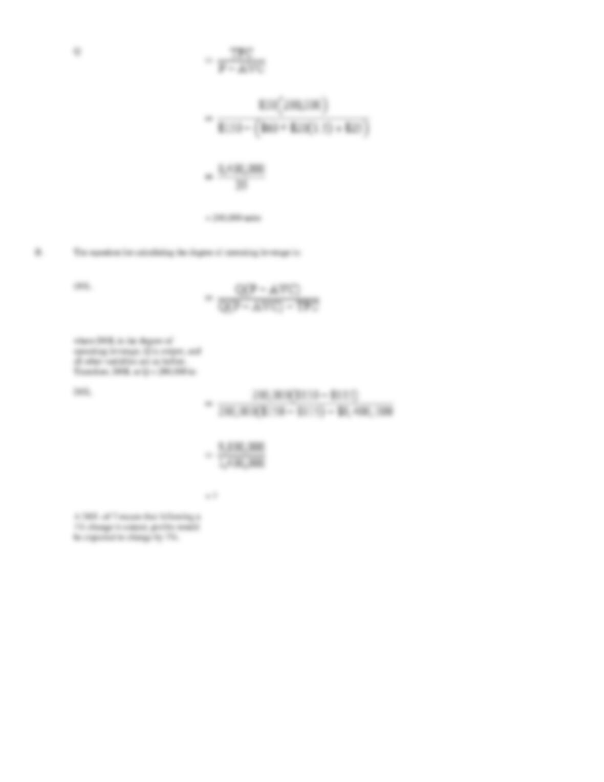
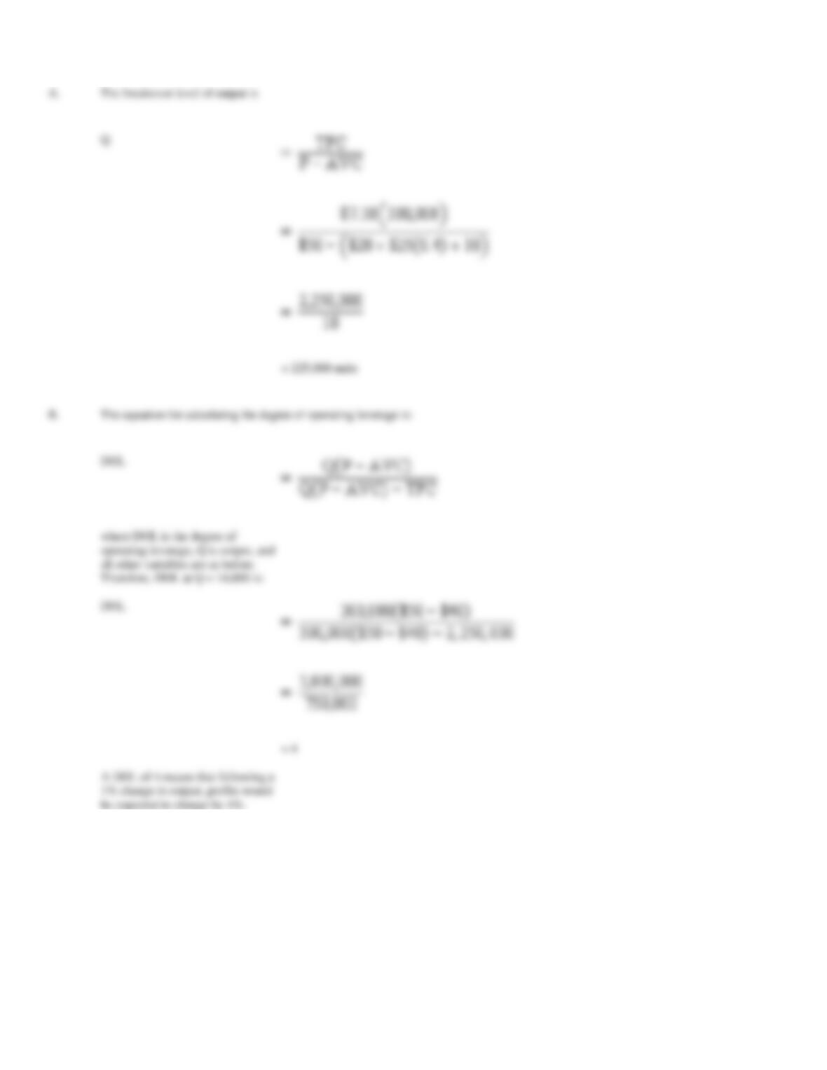
What is Ion Generating’s breakeven sales volume (in units) for smoke detectors?
B.
Calculate the degree of operating leverage at a projected volume of 300,000 units and explain what the DOL means.
43. Multiplant Operation. Tasty Snacks, Inc., a regional snack foods company (corn chips, potato chips, etc.)
in the northeast, is considering two alternative proposals for expansion into southeastern states. Alternative 1:
Construct a single plant in Chattanooga, Tennessee with a monthly production capacity of 250,000 cases, a
monthly fixed cost of $265,000, and a variable cost of $45 per case. Alternative 2: Construct three plants, one
each in Birmingham, Alabama, Tallahassee, Florida, and Charlotte, North Carolina, with capacities of 100,000,
80,000 and 70,000, respectively, and monthly fixed costs of $180,000, $150,000, and $135,000 each. Variable
costs would be only $44 per case because of lower distribution costs. To achieve these cost savings, sales from
each smaller plant would be limited to demand within its home state. The total estimated monthly sales volume
of 175,000 cases in these three southeastern states is distributed as follows: 70,000 cases in Florida, 60,000
cases in North Carolina, and 45,000 cases in Alabama.
A.
Assuming a wholesale price of $50 per case, calculate the breakeven output quantities for each alternative.
B.
At a wholesale price of $50 per case in all states, and assuming sales at the projected levels, which alternative expansion scheme
provides Tasty Snacks with the highest profit per month?
C.
If sales increase to production capacities, which alternative would prove to be more profitable?
A.
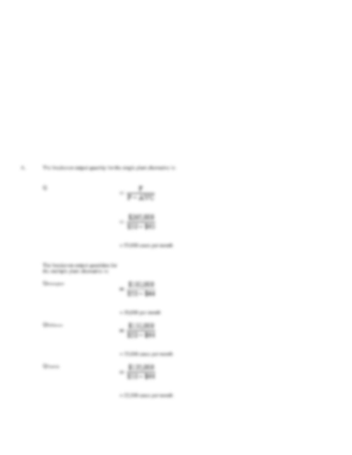
The breakeven output quantity for the single plant alternative is:
= 25,000 cases per month
44. Multiplant Operation. Nature’s Green, Inc., a manufacturer of alfalfa tablets sold in health-food stores,
currently operates just outside of Meno, California. Nature’s Green is considering two alternative proposals for
expansion, because it has run out of acreage to grow its organically-farmed alfalfa. It has found the following
sites where farmers are willing to supply organic alfalfa: Alternative 1: Construct a single plant in Big Cabin,
Oklahoma with a monthly production capacity of 50,000 cases, a monthly fixed cost of $275,000, and a variable
cost of $100 per case. Alternative 2: Construct three plants, one each in Eudora, Kansas, Springfield, Missouri,
and Tonkawa, Oklahoma, with capacities of 25,000, 20,000 and 15,000, respectively, and monthly fixed costs
of $200,000, $175,000, and $160,000 each. Variable costs would be only $95 per case because of lower
distribution costs. To achieve these cost savings, sales from each smaller plant would be limited to demand
within its home state. The total estimated monthly sales volume of 49,000 cases in these three southeastern
states is distributed as follows: 20,000 cases in Kansas, 15,000 cases in Missouri, and 14,000 cases in
Oklahoma.
A.
Assuming a wholesale price of $120 per case, calculate the breakeven output quantities for each alternative.
B.
Assuming sales at the projected levels, which alternative expansion scheme provides Nature’s Green with the highest profit per month?
C.
If sales increase to production capacities, which alternative would prove to be more profitable?
A.
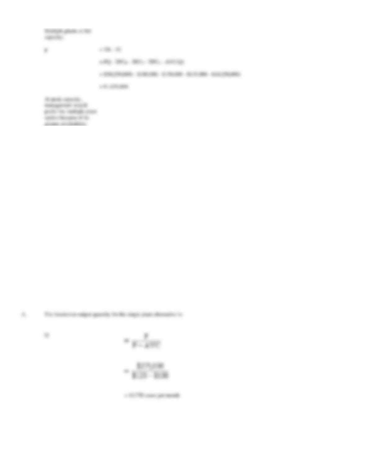
The breakeven output quantity for the single plant alternative is:
= 13,750 cases per month
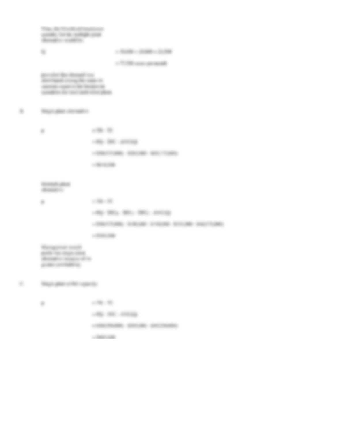
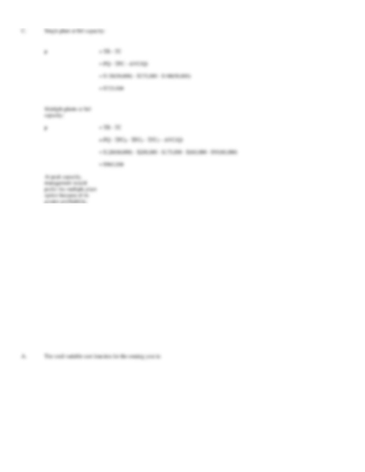
p
= TR – TC
= PQ – TFCB – TFCT – TFCC – AVC(Q)
= $50(250,000) – $180,000 – $150,000 – $135,000 – $44(250,000)
= $1,035,000
45. Learning Curve. Fashionable Designs, Ltd., plans to market a new sports blazer. Based on information
provided by the accounting department, the company estimates fixed costs of $40,000 per year and average
variable costs at:
AVC = $1 + $0.001Q
where AVC is average variable cost (in dollars) and Q is output measured in cases of output per year.
A.
Calculate total cost and average total cost for the coming year at a projected volume of 12,000 units.
B.
An increase in worker productivity due to greater experience or learning during the course of the year resulted in a substantial cost
saving for the company. Calculate the effect of learning on average total cost if actual total cost was $250,000 at an actual volume of
15,000 units.
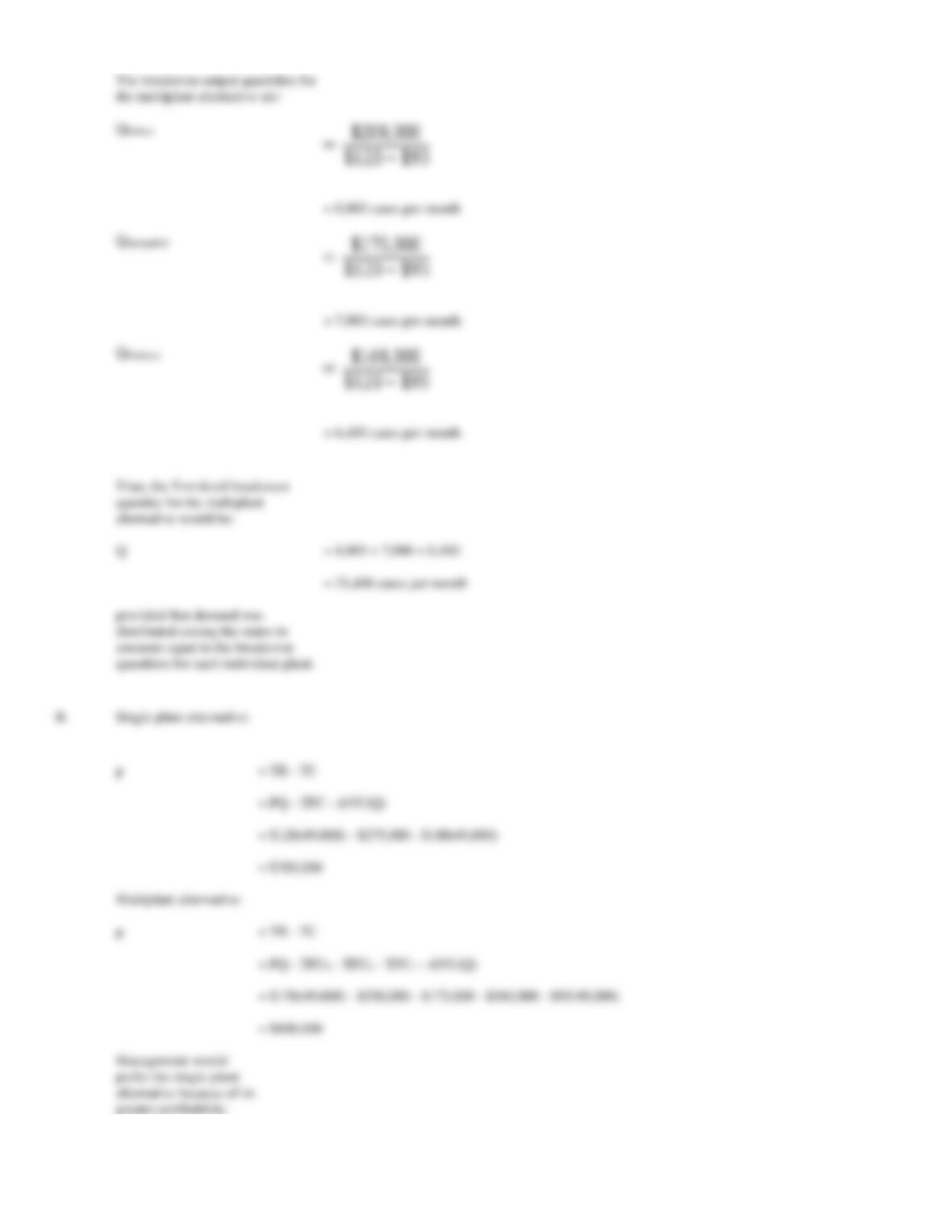
Single plant at full capacity:
p
= TR – TC
= PQ – TFC – AVC(Q)
= $120(50,000) – $275,000 – $100(50,000)
= $725,000
= PQ – TFCE – TFCS – TFCT – AVC(Q)
= $965,000
46. Learning Curve. Teddy Bear, Inc., a rapidly growing manufacturer of high fashion children’s shoes, plans
where AVC is average variable cost (in dollars) and Q is output measured in cases of output per year.
A.
Calculate total cost and average total cost for the coming year at a projected volume of 50,000 pairs of shoes.
B.
An increase in worker productivity due to greater experience or learning during the course of the year resulted in a substantial cost
saving for the company. Calculate the effect of learning on average total cost if actual total cost was $1,080,000 at an actual volume of
60,000 pairs of shoes.
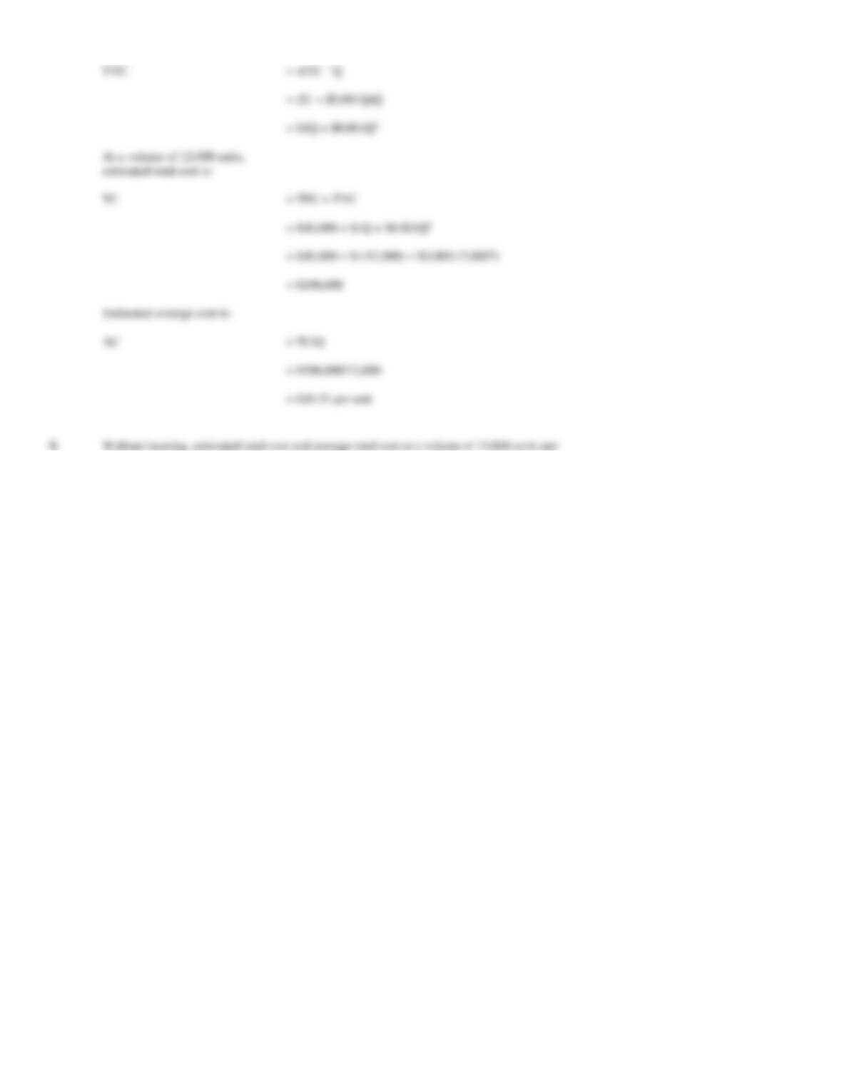
A.
The total variable cost function for the coming year is:
TVC
= AVC ´ Q
= ($5 + $0.0001Q)Q
= $1,000,000
AC
= TC/Q
= $1,000,000/50,000
= $20 per pair
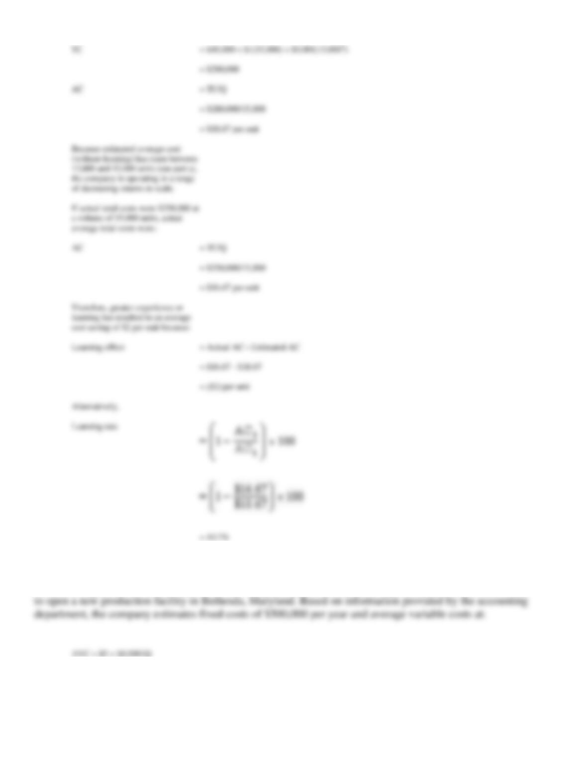
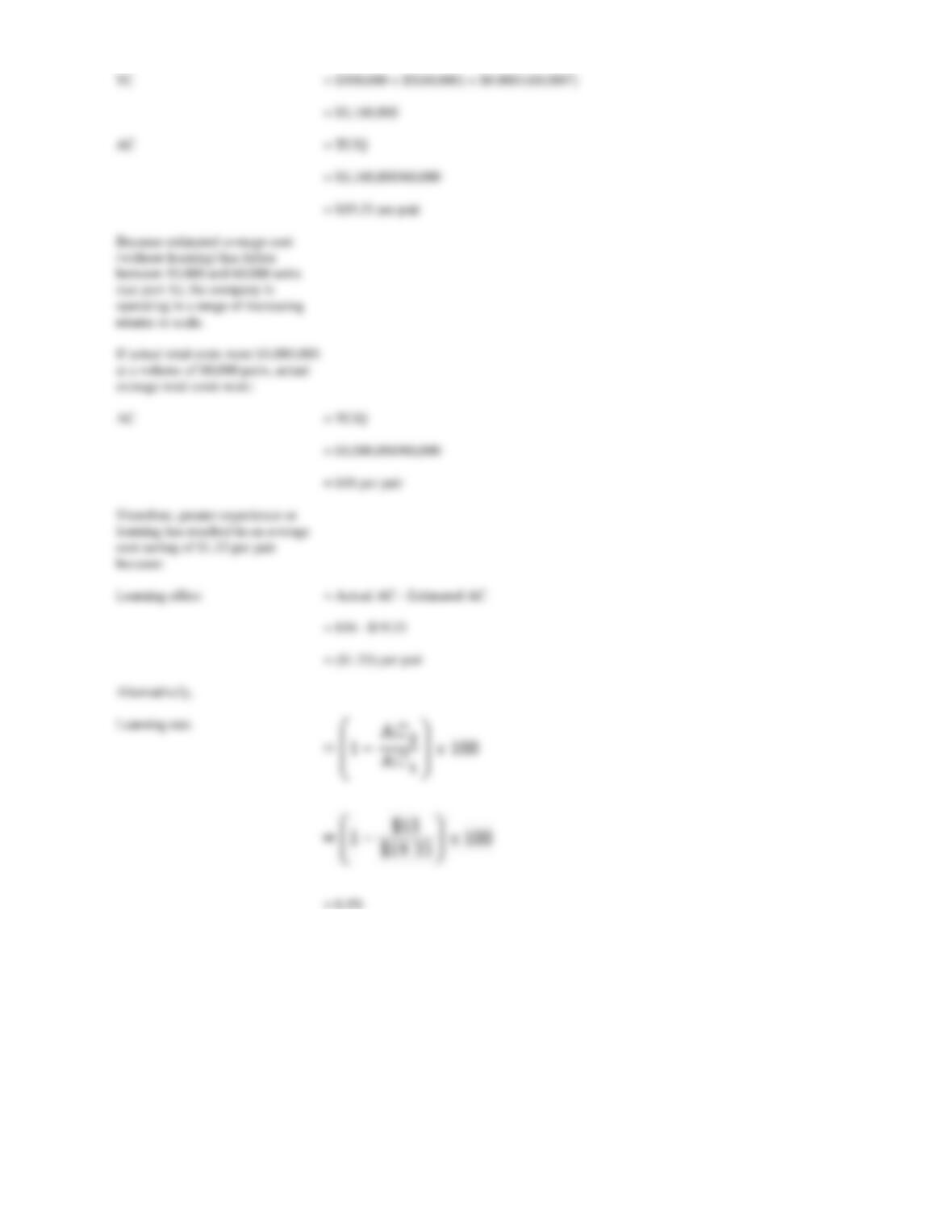
Without learning, estimated total cost and average total cost at a volume of 60,000 pairs are:
47. Economies of Scale. Tucson Timing, Inc., has just completed a study of weekly production costs during the
past year for its premium quality, automotive strobe timing light, the Flash Gun II. By regressing total variable
costs on output the firm estimated the following equation.
TVC
= $30 + $125Q – $1Q2
(15) (3) (0.5)
R2
= 90%, SEE = 10
= $1,160,000
= TC/Q
= $1,160,000/60,000
= $19.33 per pair
= $1,080,000/60,000
because:
Learning effect
= Actual AC – Estimated AC
= ($1.33) per pair
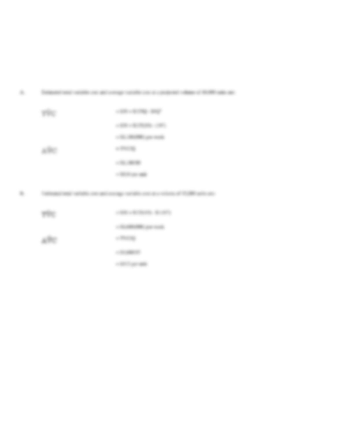
Here total variable cost (TVC) is expressed in thousands of dollars and Q is in thousands of strobe timing lights (units) produced per week. Numbers
in parentheses are the standard errors of the coefficients.
A.
Estimate total variable cost and average variable cost per week for the coming year at a projected volume of 10,000 units per week.
B.
During this period, the company experienced an unexpected interruption in supplier deliveries, and unexpected increases in the cost of
labor and materials. If actual average variable costs were $100 per unit at an average actual volume of 15,000 units per week, calculate
the separate influences on average variable cost of lost economies of scale and the unexpected input cost increases.
A.
Estimated total variable cost and average variable cost at a projected volume of 10,000 units are:
= $1,180(000) per week
= $1,180/10
Estimated total variable cost and average variable cost at a volume of 15,000 units are:
= $1,680(000) per week
= $1,680/15
= $112 per unit
48. Economies of Scale. Windy Manes, Inc., has just completed a study of weekly production costs during the
past year for its compact hand-held hair dryer. By regressing total variable costs on output the firm estimated
the following equation.
TVC
= $15 + $5Q – $0.01Q2
(4) (2) (0.005)
R2
= 83.5%, SEE = 18
Here total variable cost (TVC) is expressed in thousands of dollars and Q is in thousands of hand-held hair dryers (units) produced per week.
Numbers in parentheses are the standard errors of the coefficients.
A.
Estimate total variable cost and average variable cost per week for the coming year at a projected volume of 50,000 units per week.
B.
During this period, the company experienced an unexpected interruption in supplier deliveries, and unexpected increases in the cost of
labor and materials. If actual average variable costs were $4.30 per unit at an average actual volume of 75,000 units per week, calculate
the separate influences on average variable cost of lost economies of scale and the unexpected input cost increases.
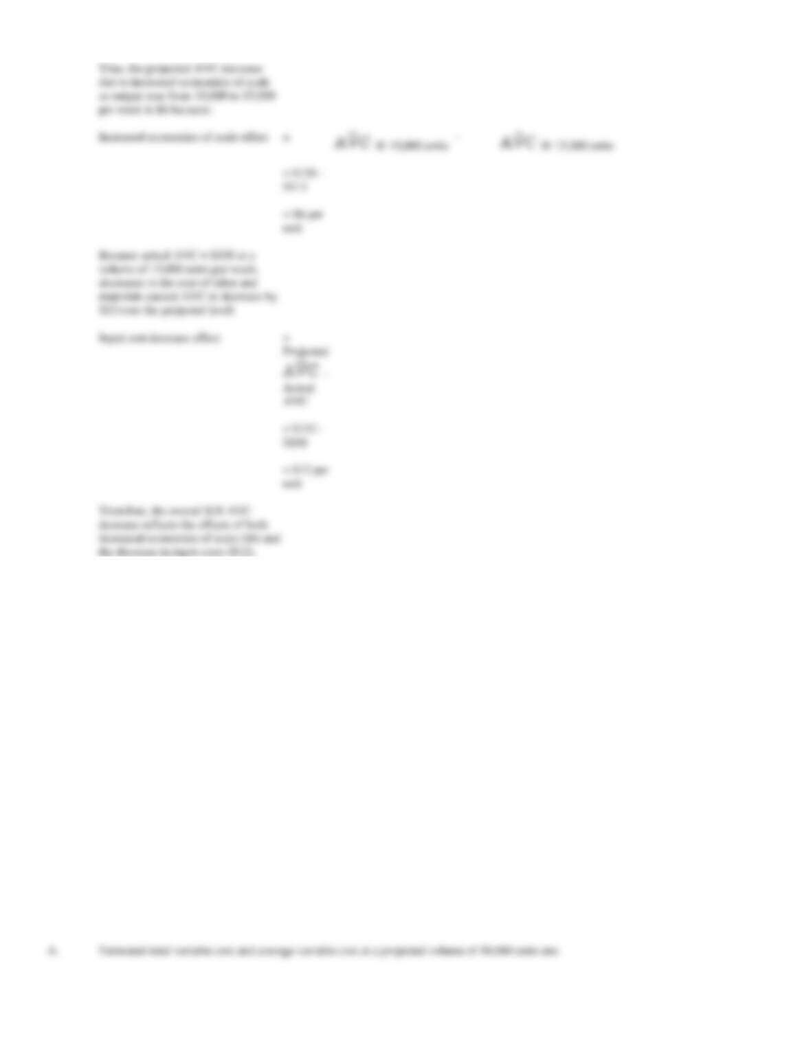
A.
Estimated total variable cost and average variable cost at a projected volume of 50,000 units are:
the decrease in input costs ($12).
49. Cost Estimation. Natural Gas, Inc., has just completed a cost study of its natural gas production operation.
By regressing total variable costs (in $000) per week on gas output, the following equation was estimated:
Total variable cost
= $6,500 + $0.25Q – $0.000125Q2
(5,000) (0.12) (0.00005)
Here Q is natural gas production in thousand cubic feet (units) and the numbers in parentheses are the standard errors of the coefficients. The R2 for
the equation is 85%, and the standard error of the estimate is 50 for the weekly observations over a two-year period.
A.
Interpret the coefficient of determination (R2).
B.
If volume averages 8,000 units per week, calculate the range within which we would expect to find actual total variable and average
variable costs with 95% confidence.
C.
Calculate and interpret relevant t statistics.
D.
Are Natural Gas’ average variable costs per unit increasing as output expands?
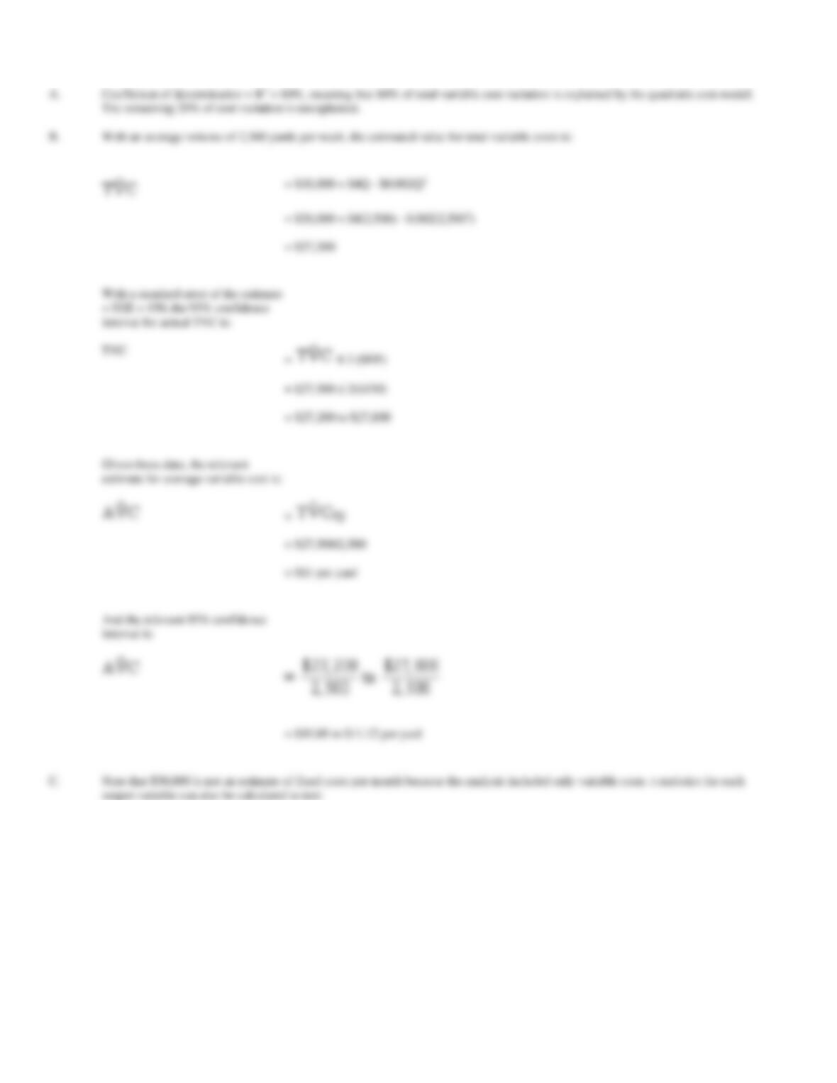
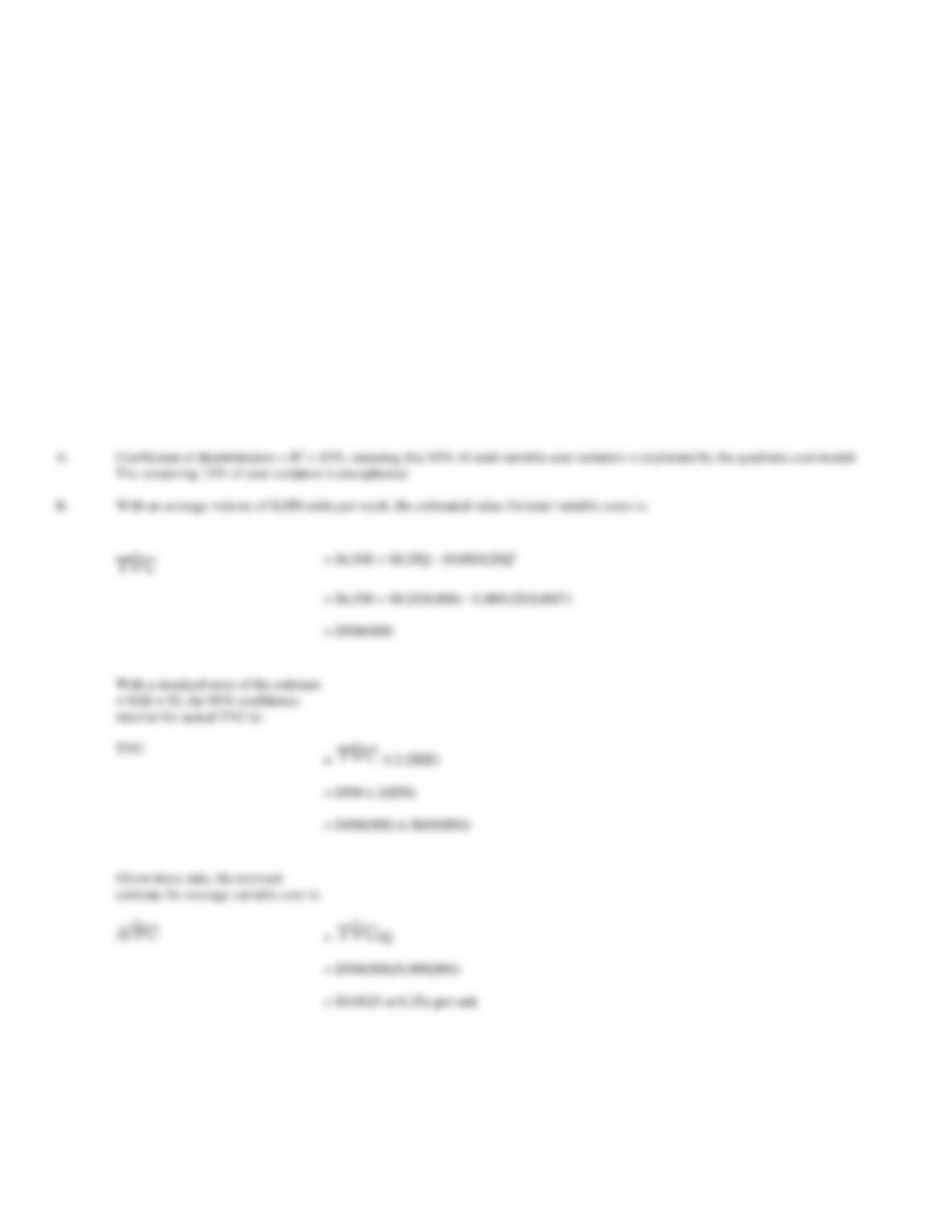
The remaining 15% of cost variation is unexplained.
With an average volume of 8,000 units per week, the estimated value for total variable costs is:
= $6,500 + $0.25(8,000) – 0.000125(8,0002)
= $500(000)
= $500 2($50)
= $400(000) to $600(000)
= $500(000)/8,000(000)
= $0.0625 or 6.25¢ per unit
50. Cost Estimation. Hampshire Textiles, Inc., has just completed a cost study of its moire taffeta production
facility. By regressing total variable costs per week on cloth output, one of their financial analysts estimated the
following equation:
Total variable cost
= $30,000 + $4Q – $0.002Q2
(20,000) (1.5) (0.0008)
Here Q is moire taffeta cloth production in square yards and the numbers in parentheses are the standard errors of the coefficients. The R2 for the
equation was 80%, and the standard error of the estimate was 150 for the weekly observations over a two-year period.
A.
Interpret the coefficient of determination (R2).
B.
If volume averages 2,500 yards per week, calculate the range within which we would expect to find actual total variable and average
variable costs with 95% confidence.
C.
Calculate and interpret relevant t-statistics.
D.
Are Hampshire Textiles’ average variable costs per unit increasing as output expands?
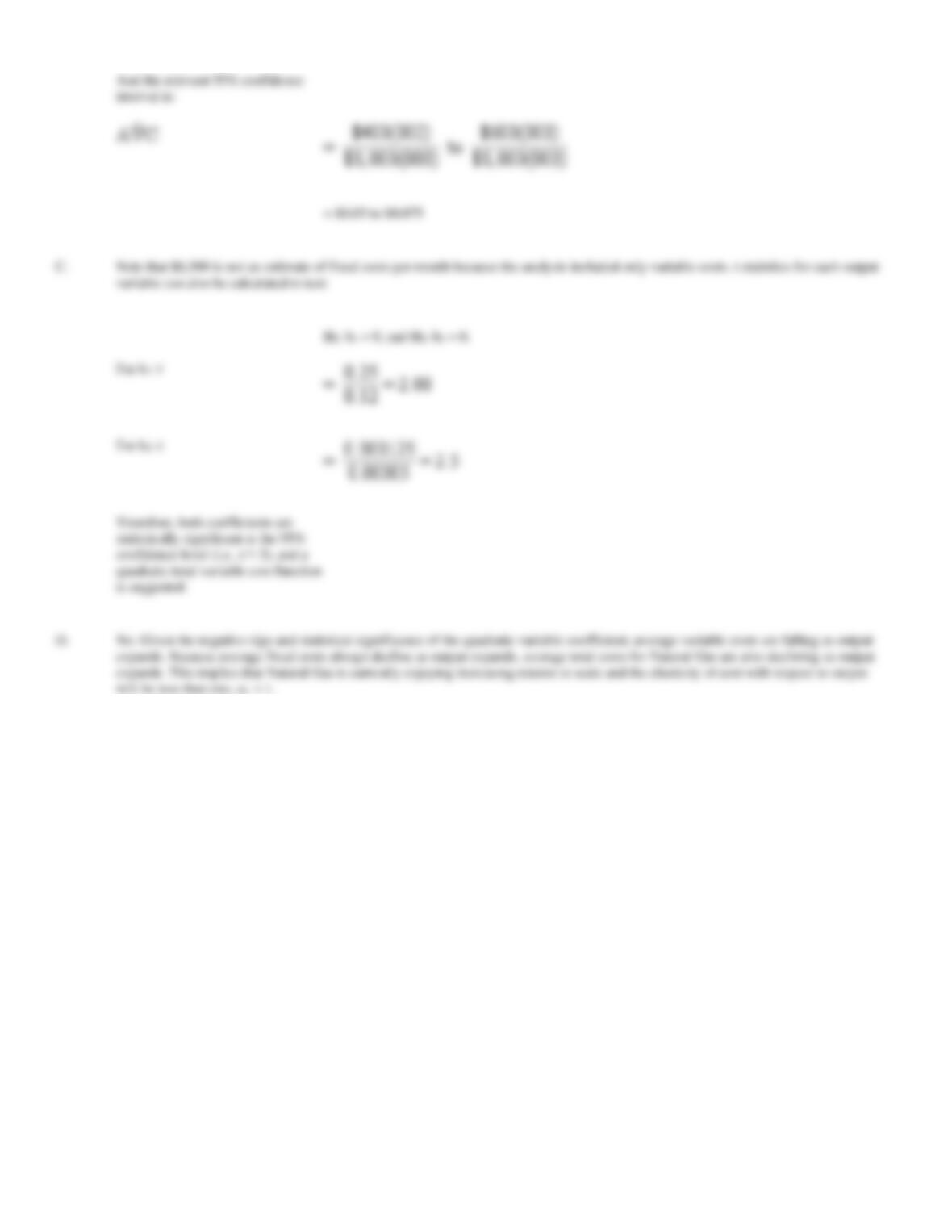
And the relevant 95% confidence
= $0.05 to $0.075
C.
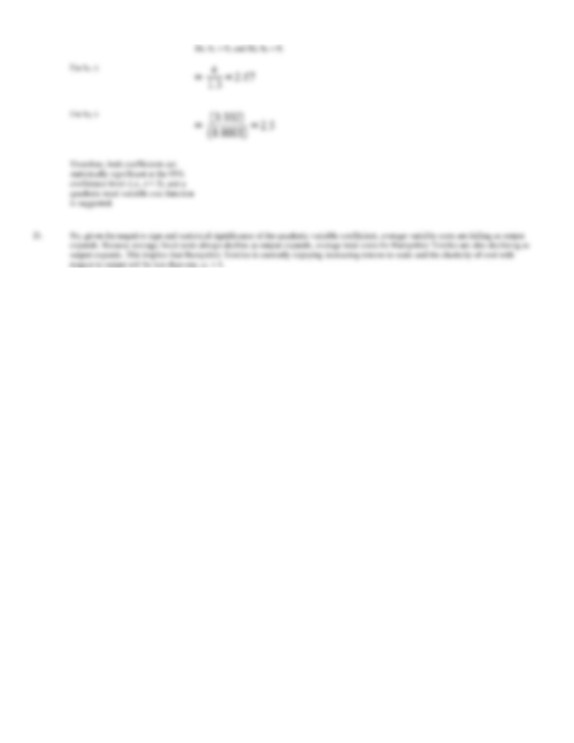
Note that $6,500 is not an estimate of fixed costs per month because the analysis included only variable costs. t statistics for each output
will be less than one, eC < 1.