5) In the case of perfect multicollinearity, OLS is unable to estimate the slope coefficients of the variables
involved. Assume that you have included both X1 and X2 as explanatory variables, and that X2 = X, so
that there is an exact relationship between two explanatory variables. Does this pose a problem for
estimation?
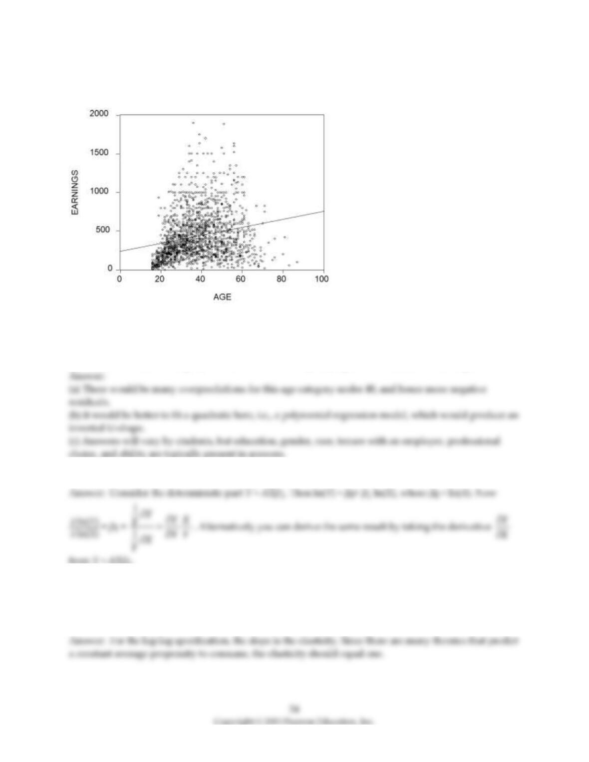
6) The figure shows is a plot and a fitted linear regression line of the age-earnings profile of 1,744
individuals, taken from the Current Population Survey.
(a) Describe the problems in predicting earnings using the fitted line. What would the pattern of the
residuals look like for the age category under 40?
(b) What alternative functional form might fit the data better?
(c) What other variables might you want to consider in specifying the determinants of earnings?
7) (Requires Calculus) Show that for the log-log model the slope coefficient is the elasticity.
8) Assume that you had data for a cross-section of 100 households with data on consumption and
personal disposable income. If you fit a linear regression function regressing consumption on disposable
income, what prior expectations do you have about the slope and the intercept? The slope of this
regression function is called the “marginal propensity to consume.” If, instead, you fit a log-log model,
then what is the interpretation of the slope? Do you have any prior expectation about its size?
9) The textbook shows that ln(x + Δx) – ln(x) ≅ . Show that this is equivalent to the following
approximation ln(1 + y) ≅ y if y is small. You use this idea to estimate a demand for money function,
which is of the form m = β0 × ×, × eu where m is the quantity of (real) money, GDP is the
value of (real) Gross Domestic Product, and R is the nominal interest rate. You collect the quarterly data
from the Federal Reserve Bank of St. Louis data bank (“FRED”), which lists the money supply and GDP in
billions of dollars, prices as an index, and nominal interest rates in percentage points per year
You generate the variables in your regression program as follows: m = (money supply)/price index; GDP =
(Gross Domestic Product/Price Index), and R = nominal interest rate in percentage points per annum.
Next you perform the log-transformations on the real money supply, real GDP, and on (1+R). Can you for
see a problem in using this transformation?
10) You have estimated an earnings function, where you regressed the log of earnings on a set of
continuous explanatory variables (in levels) and two binary variables, one for gender and the other for
marital status. One of the explanatory variables is education.
(a) Interpret the education coefficient.
(b) Next, specify the binary variables and an equation, where the default is a single male, without
allowing for interaction between marital status and gender. Indicate the coefficients that measure the
effect of a single male, single female, married male, and married female.
(c) Finally allow for an interaction between the gender and marital status binary variables. Repeat the
exercise of writing down the various effects based on the female/male and single/married status. Why is
the latter approach more general than the former?
11) You have been told that the money demand function in the United States has been unstable since the
late 1970. To investigate this problem, you collect data on the real money supply (m=M/P; where M is M1
and P is the GDP deflator), (real) gross domestic product (GDP) and the nominal interest rate (R). Next
you consider estimating the demand for money using the following alternative functional forms:
(i) m = β0 + β1 × GDP + β2 x R+ u
(ii) m = β0 × x × eu
(iii) m = β0 × x × eu
Give an interpretation for β1 and β2 in each case. How would you calculate the income elasticity in case
(i)?
12) You have collected data for a cross-section of countries in two time periods, 1960 and 1997, say. Your
task is to find the determinants for the Wealth of a Nation (per capita income) and you believe that there
are three major determinants: investment in physical capital in both time periods (X1,T and X1,0),
investment in human capital or education (X2,T and X2,0), and per capita income in the initial period
(Y0). You run the following regression:
ln(YT) = β0 + β1X1,T + β2X1,0 + β3X2,T + β4X1,0 + ln(Y0) + uT
One of your peers suggests that instead, you should run the growth rate in per capita income over the
two periods on the change in physical and human capital. For those results to be a parsimonious
presentation of your initial regression, what three restrictions would have to hold? How would you test
for these? The same person also points out to you that the intercept vanishes in equations where the data
is differenced. Is that true?
13) Earnings functions attempt to predict the log of earnings from a set of explanatory variables, both
binary and continuous. You have allowed for an interaction between two continuous variables: education
and tenure with the current employer. Your estimated equation is of the following type:
= 0 + 1 × Femme + 2 × Educ + 3 × Tenure + 4 x (Educ × Tenure) + ∙∙∙
where Femme is a binary variable taking on the value of one for females and is zero otherwise, Educ is the
number of years of education, and tenure is continuous years of work with the current employer. What is
the effect of an additional year of education on earnings (“returns to education”) for men? For women? If
you allowed for the returns to education to differ for males and females, how would you respecify the
above equation? What is the effect of an additional year of tenure with a current employer on earnings?
14) Many countries that experience hyperinflation do not have market-determined interest rates. As a
result, some authors have substituted future inflation rates into money demand equations of the
following type as a proxy:
(m is real money, and P is the consumer price index).
Income is typically omitted since movements in it are dwarfed by money growth and the inflation rate.
Authors have then interpreted β1 as the “semi-elasticity” of the inflation rate. Do you see any problems
with this interpretation?
15) To investigate whether or not there is discrimination against a sub-group of individuals, you regress
the log of earnings on determining variables, such as education, work experience, etc., and a binary
variable which takes on the value of one for individuals in that sub-group and is zero otherwise. You
consider two possible specifications. First you run two separate regressions, one for the observations that
include the sub-group and one for the others. Second, you run a single regression, but allow for a binary
variable to appear in the regression. Your professor suggests that the second equation is better for the
task at hand, as long as you allow for a shift in both the intercept and the slopes. Explain her reasoning.

16) Being a competitive female swimmer, you wonder if women will ever be able to beat the time of the
male gold medal winner. To investigate this question, you collect data for the Olympic Games since 1910.
At first you consider including various distances, a binary variable for Mark Spitz, and another binary
variable for the arrival and presence of East German female swimmers, but in the end decide on a simple
linear regression. Your dependent variable is the ratio of the fastest women’s time to the fastest men’s
time in the 100 m backstroke, and the explanatory variable is the year of the Olympics. The regression
result is as follows,
= 4.42 – 0.0017 × Olympics,
where TFoverM is the relative time of the gold medal winner, and Olympics is the year of the Olympic
Games. What is your prediction when females will catch up to men in this discipline? Does this sound
plausible? What other functional form might you want to consider?
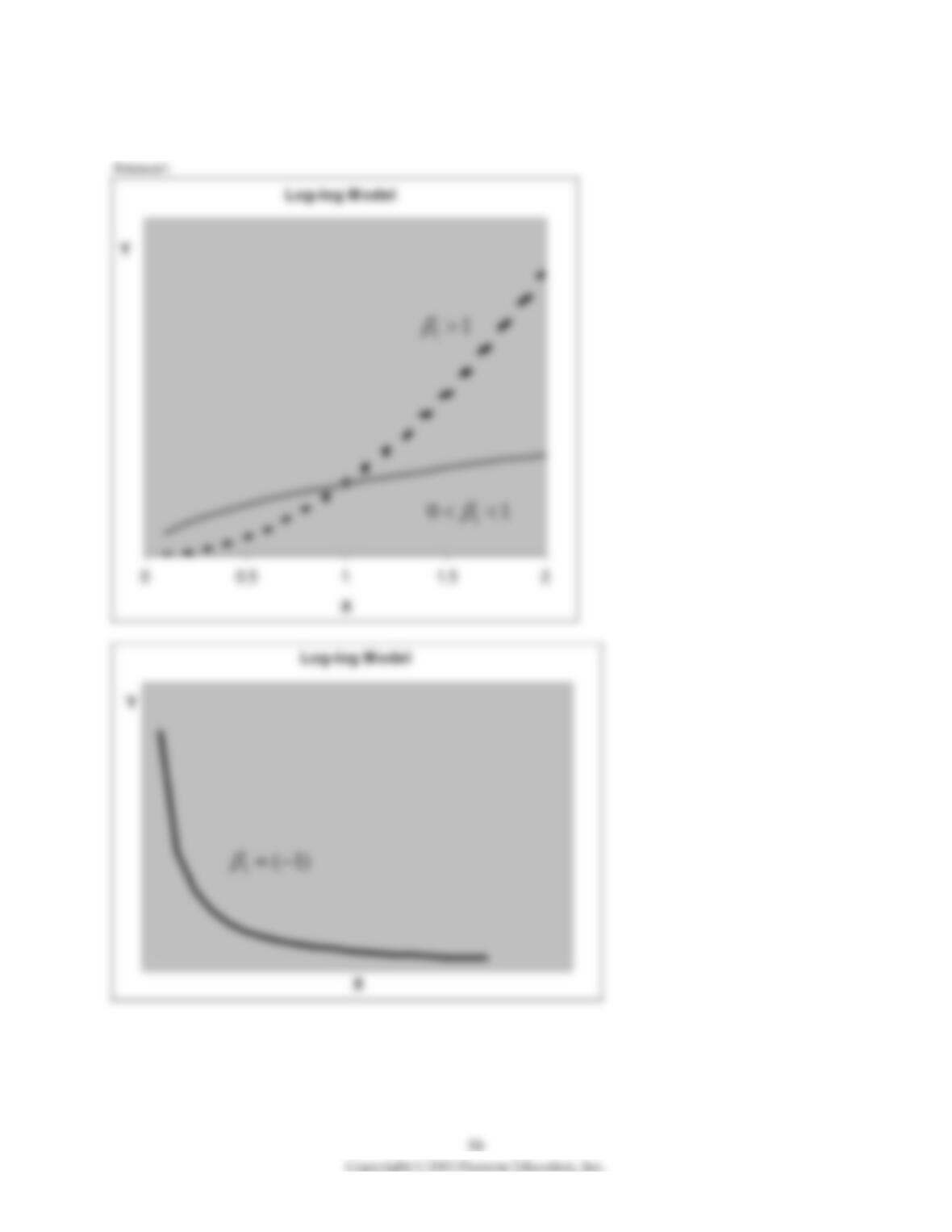
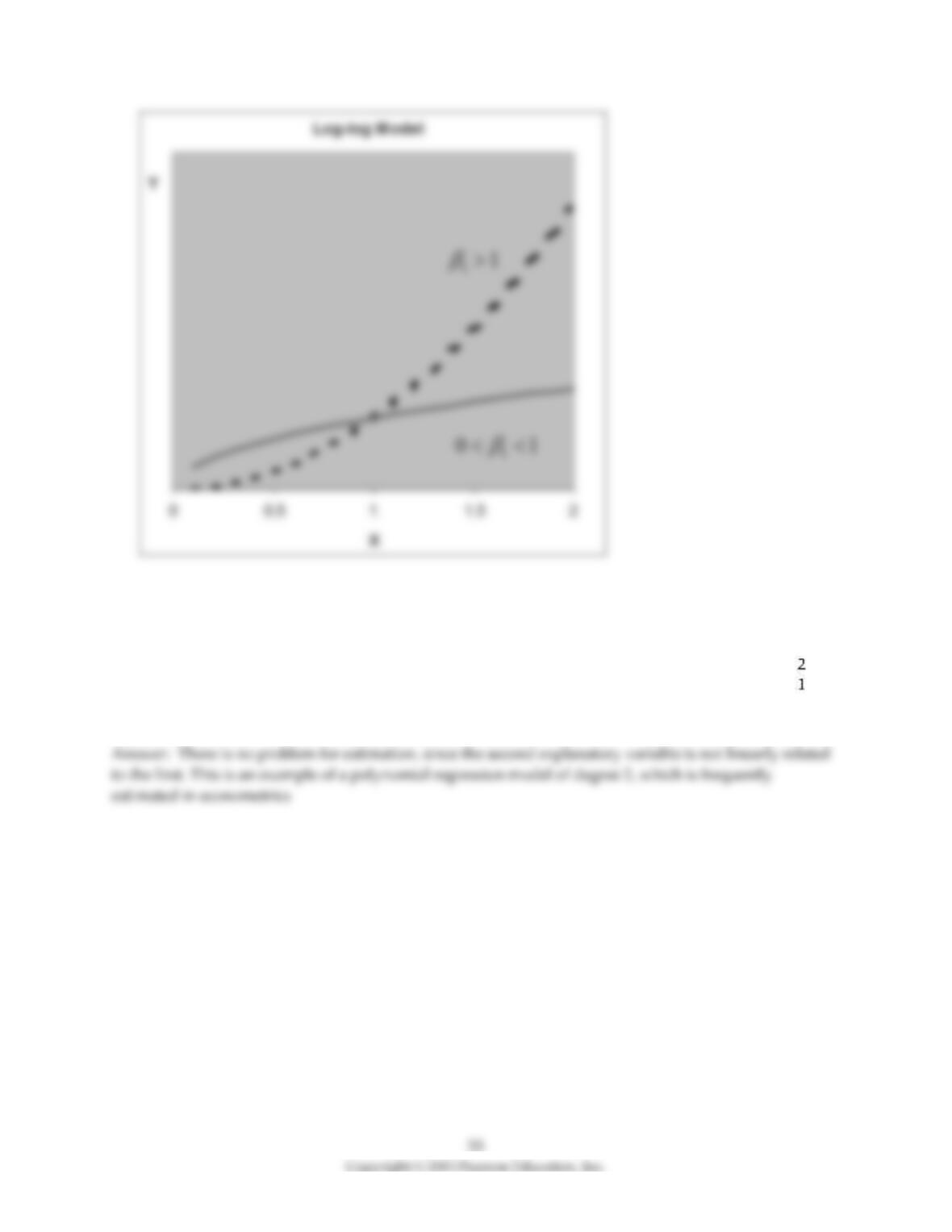
17) Sketch for the log-log model what the relationship between Y and X looks like for various parameter
values of the slope, i.e., β1 > 1; 0 < β1 < 1; β1 = (-1).
18) Show that for the following regression model
Yt =
where t is a time trend, which takes on the values 1, 2, …,T, β1 represents the instantaneous (“continuous
compounding”) growth rate. Show how this rate is related to the proportionate rate of growth, which is
calculated from the relationship
Yt = Y0 × (1 + g)t
when time is measured in discrete intervals.
19) Your task is to estimate the ice cream sales for a certain chain in New England. The company makes
available to you quarterly ice cream sales (Y) and informs you that the price per gallon has approximately
remained constant over the sample period. You gather information on average daily temperatures (X)
during these quarters and regress Y on X, adding seasonal binary variables for spring, summer, and fall.
These variables are constructed as follows: DSpring takes on a value of 1 during the spring and is zero
otherwise, DSummer takes on a value of 1 during the summer, etc. Specify three regression functions
where the following conditions hold: the relationship between Y and X is (i) forced to be the same for
each quarter; (ii) allowed to have different intercepts each season; (iii) allowed to have varying slopes and
intercepts each season. Sketch the difference between (i) and (ii). How would you test which model fits
the data the best?
20) In estimating the original relationship between money wage growth and the unemployment rate,
Phillips used United Kingdom data from 1861 to 1913 to fit a curve of the following functional form
( + β0) = β1 × × eu,
where is the percentage change in money wages and ur is the unemployment rate. Sketch the
function. What role does β0 play? Can you find a linear transformation that allows you to estimate the
above function using OLS? If, after taking logarithms on both sides of the equation, you tried to estimate
β1 and β2 using OLS by choosing different values for β0 by “trial and error procedure” (Phillips’s words),
what sort of problem might you run into with the left-hand side variable for some of the observations?
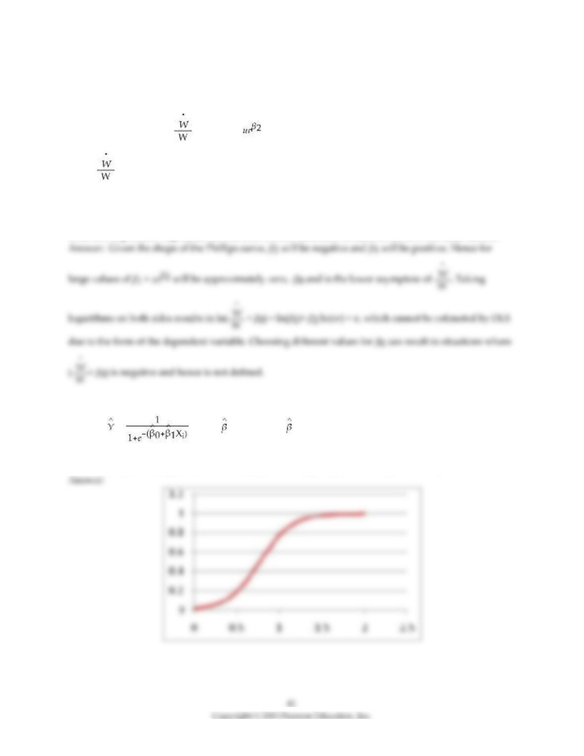
21) Using a spreadsheet program such as Excel, plot the following logistic regression function with a
single X, i = , where 0 = – 4.13 and 1 = 5.37. Enter values of X in the first column starting
from 0 and then incrementing these by 0.1 until you reach 2.0. Then enter the logistic function formula in
the next column. Finally produce a scatter plot, connecting the predicted values with a line.
22) Table 8.1 on page 284 of your textbook displays the following estimated earnings function in column
(4):
= 1.503 + 0.1032 × educ – 0.451 × DFemme + 0.0143 × (DFemme×educ)
(0.023) (0.0012) (0.024) (0.0017)
+ 0.0232 × exper – 0.000368 × exper2 – 0.058 × Midwest – 0.0098 × South – 0.030 × West
(0.0012) (0.000023) (0.006) (0.006) (0.007)
n = 52.790, 2 = 0.267
Given that the potential experience variable (exper) is defined as (Age-Education-6) find the age at which
individuals with a high school degree (12 years of education) and with a college degree (16 years of
education) have maximum earnings, holding all other factors constant.
23) Consider a typical beta convergence regression function from macroeconomics, where the growth of a
country’s per capita income is regressed on the initial level of per capita income and various other
economic and socio-economic variables. Assume that two of these variables are the average number of
years of education in the specific country and a binary variable which indicates whether or not the
country experienced a significant number of years of civil war/unrest. Explain why it would make sense
to have these two variables enter separately and also why you should use an interaction term. What signs
would you expect on the three coefficients?

43
24) Consider the following regression of testscores on an intercept, a binary variable that equals 1 if the
student-teacher ratio is 20 or more (HiSTR) and another binary variable that equals 1 if the percentage of
English learners is 10% or more (HiEL).
= 664/1 – 1.9 × HiSTR – 18.2×HiEL – 3.5 × (HiSTR × HiEL)
Using the two by two table below, fill in the expected testscores of a student with various combinations of
the high/low student teacher ratio and the high/low percent of English learners.
STR < 20
STR 20
EL < 10%
EL 10%
EL < 10%
664.1
662.2
EL 10%
645.9
640.5