1
Introduction to Econometrics, 3e (Stock)
Chapter 8 Nonlinear Regression Functions
8.1 Multiple Choice
1) In nonlinear models, the expected change in the dependent variable for a change in one of the
explanatory variables is given by
A)
△
Y = f(X1 + X1, X2,… Xk).
B)
△
Y = f(X1 +
△
X1, X2 + △X2,…, Xk+ △Xk)- f(X1, X2,…Xk).
C)
△
Y = f(X1 +
△
X1, X2,…, Xk)- f(X1, X2,…Xk).
D)
△
Y = f(X1 + X1, X2,…, Xk)- f(X1, X2,…Xk).
2) The interpretation of the slope coefficient in the model Yi = β0 + β1 ln(Xi) + ui is as follows:
A) a 1% change in X is associated with a β1 % change in Y.
B) a 1% change in X is associated with a change in Y of 0.01 β1.
C) a change in X by one unit is associated with a β1 100% change in Y.
D) a change in X by one unit is associated with a β1 change in Y.
3) The interpretation of the slope coefficient in the model ln(Yi) = β0 + β1Xi + ui is as follows:
A) a 1% change in X is associated with a β1 % change in Y.
B) a change in X by one unit is associated with a 100 β1 % change in Y.
C) a 1% change in X is associated with a change in Y of 0.01 β1.
D) a change in X by one unit is associated with a β1 change in Y.
4) The interpretation of the slope coefficient in the model ln(Yi) = β0 + β1 ln(Xi)+ ui is as follows:
A) a 1% change in X is associated with a β1 % change in Y.
B) a change in X by one unit is associated with a β1 change in Y.
C) a change in X by one unit is associated with a 100 β1 % change in Y.
D) a 1% change in X is associated with a change in Y of 0.01 β1.

5) In the case of regression with interactions, the coefficient of a binary variable should be interpreted as
follows:
A) there are really problems in interpreting these, since the ln(0) is not defined.
B) for the case of interacted regressors, the binary variable coefficient represents the various intercepts for
the case when the binary variable equals one.
C) first set all explanatory variables to one, with the exception of the binary variables. Then allow for each
of the binary variables to take on the value of one sequentially. The resulting predicted value indicates
the effect of the binary variable.
D) first compute the expected values of Y for each possible case described by the set of binary variables.
Next compare these expected values. Each coefficient can then be expressed either as an expected value
or as the difference between two or more expected values.
6) The following interactions between binary and continuous variables are possible, with the exception of
A) Yi = β0 + β1Xi + β2Di + β3(Xi × Di) + ui.
B) Yi = β0 + β1Xi + β2(Xi × Di) + ui.
C) Yi = (β0 + Di) + β1Xi + ui.
D) Yi = β0 + β1Xi + β2Di + ui.
7) An example of the interaction term between two independent, continuous variables is
A) Yi = β0 + β1Xi + β2Di + β3(Xi × Di) + ui.
B) Yi = β0 + β1X1i + β2X2i + ui.
C) Yi = β0 + β1D1i + β2D2i + β3 (D1i × D2i) + ui.
D) Yi = β0 + β1X1i + β2X2i + β3(X1i × X2i) + ui.
8) Including an interaction term between two independent variables, X1 and X2, allows for the following
except:
A) the interaction term lets the effect on Y of a change in X1 depend on the value of X2.
B) the interaction term coefficient is the effect of a unit increase in X1 and X2 above and beyond the sum
of the individual effects of a unit increase in the two variables alone.
C) the interaction term coefficient is the effect of a unit increase in .
D) the interaction term lets the effect on Y of a change in X2 depend on the value of X1.
9) A nonlinear function
A) makes little sense, because variables in the real world are related linearly.
B) can be adequately described by a straight line between the dependent variable and one of the
explanatory variables.
C) is a concept that only applies to the case of a single or two explanatory variables since you cannot
draw a line in four dimensions.
D) is a function with a slope that is not constant.

10) An example of a quadratic regression model is
A) Yi = β0 + β1X + β2Y2 + ui.
B) Yi = β0 + β1ln(X) + ui.
C) Yi = β0 + β1X + β2X2 + ui.
D) = β0 + β1X + ui.
11) (Requires Calculus) In the equation = 607.3 + 3.85 Income – 0.0423Income2, the following
income level results in the maximum test score
A) 607.3.
B) 91.02.
C) 45.50.
D) cannot be determined without a plot of the data.
12) To decide whether Yi = β0 + β1X + ui or ln(Yi) = β0 + β1X + ui fits the data better, you cannot consult
the regression R2 because
A) ln(Y) may be negative for 0<Y<1.
B) the TSS are not measured in the same units between the two models.
C) the slope no longer indicates the effect of a unit change of X on Y in the log-linear model.
D) the regression R2 can be greater than one in the second model.
13) You have estimated the following equation:
= 607.3 + 3.85 Income – 0.0423 Income2,
where TestScore is the average of the reading and math scores on the Stanford 9 standardized test
administered to 5th grade students in 420 California school districts in 1998 and 1999. Income is the
average annual per capita income in the school district, measured in thousands of 1998 dollars. The
equation
A) suggests a positive relationship between test scores and income for most of the sample.
B) is positive until a value of Income of 610.81.
C) does not make much sense since the square of income is entered.
D) suggests a positive relationship between test scores and income for all of the sample.

14) A polynomial regression model is specified as:
A) Yi = β0 + β1Xi + β2X+ ∙∙∙ + βrX + ui.
B) Yi = β0 + β1Xi + βXi + ∙∙∙ + βXi + ui.
C) Yi = β0 + β1Xi + β2Y+ ∙∙∙ + βrY + ui.
D) Yi = β0 + β1X1i + β2X2 + β3 (X1i × X2i) + ui.
15) For the polynomial regression model,
A) you need new estimation techniques since the OLS assumptions do not apply any longer.
B) the techniques for estimation and inference developed for multiple regression can be applied.
C) you can still use OLS estimation techniques, but the t-statistics do not have an asymptotic normal
distribution.
D) the critical values from the normal distribution have to be changed to 1.962, 1.963, etc.
16) To test whether or not the population regression function is linear rather than a polynomial of order r,
A) check whether the regression R2 for the polynomial regression is higher than that of the linear
regression.
B) compare the TSS from both regressions.
C) look at the pattern of the coefficients: if they change from positive to negative to positive, etc., then the
polynomial regression should be used.
D) use the test of (r-1) restrictions using the F-statistic.
17) The best way to interpret polynomial regressions is to
A) take a derivative of Y with respect to the relevant X.
B) plot the estimated regression function and to calculate the estimated effect on Y associated with a
change in X for one or more values of X.
C) look at the t-statistics for the relevant coefficients.
D) analyze the standard error of estimated effect.
18) The exponential function
A) is the inverse of the natural logarithm function.
B) does not play an important role in modeling nonlinear regression functions in econometrics.
C) can be written as exp(ex).
D) is ex, where e is 3.1415….

5
19) The following are properties of the logarithm function with the exception of
A) ln(1/ x) = -ln(x).
B) ln(a + x) = ln(a) + ln(x).
C) ln(ax) = ln(a) + ln(x).
D) ln(xa) a ln(x).
20) The binary variable interaction regression
A) can only be applied when there are two binary variables, but not three or more.
B) is the same as testing for differences in means.
C) cannot be used with logarithmic regression functions because ln(0) is not defined.
D) allows the effect of changing one of the binary independent variables to depend on the value of the
other binary variable.
21) In the regression model Yi = β0 + β1Xi + β2Di + β3(Xi × Di) + ui, where X is a continuous variable and
D is a binary variable, β3
A) indicates the slope of the regression when D=1.
B) has a standard error that is not normally distributed even in large samples since D is not a normally
distributed variable.
C) indicates the difference in the slopes of the two regressions.
D) has no meaning since (Xi × Di) = 0 when Di = 0.
22) In the regression model Yi = β0 + β1Xi + β2Di + β3(Xi × Di) + ui, where X is a continuous variable and
D is a binary variable, β2
A) is the difference in means in Y between the two categories.
B) indicates the difference in the intercepts of the two regressions.
C) is usually positive.
D) indicates the difference in the slopes of the two regressions.
23) In the regression model Yi = β0 + β1Xi + β2Di + β3(Xi × Di) + ui, where X is a continuous variable and
D is a binary variable, to test that the two regressions are identical, you must use the
A) t-statistic separately for β2 = 0, β2 = 0.
B) F-statistic for the joint hypothesis that β0 = 0, β1 = 0.
C) t-statistic separately for β3 = 0.
D) F-statistic for the joint hypothesis that β2 = 0, β3= 0.

6
24) In the model Yi = β0 + β1X1 + β2X2 + β3(X1 × X2) + ui, the expected effect is
A) β1 + β3X2.
B) β1.
C) β1 + β3.
D) β1 + β3X1.
25) In the log-log model, the slope coefficient indicates
A) the effect that a unit change in X has on Y.
B) the elasticity of Y with respect to X.
C) ΔY / ΔX.
D) × .
26) In the model ln(Yi) = β0 + β1Xi + ui, the elasticity of E(Y|X) with respect to X is
A) β1X
B) β1
C)
D) Cannot be calculated because the function is non-linear
27) Assume that you had estimated the following quadratic regression model
= 607.3 + 3.85 Income – 0.0423 Income2. If income increased from 10 to 11 ($10,000 to $11,000), then
the predicted effect on testscores would be
A) 3.85
B) 3.85-0.0423
C) Cannot be calculated because the function is non-linear
D) 2.96
28) Consider the polynomial regression model of degree Yi = β0 + β1Xi + β2+ …+ βr + ui. According
to the null hypothesis that the regression is linear and the alternative that is a polynomial of degree r
corresponds to
A) H0: βr = 0 vs. βr ≠ 0
B) H0: βr = 0 vs. β1 ≠ 0
C) H0: β3 = 0, …, βr = 0, vs. H1: all βj ≠ 0, j = 3, …, r
D) H0: β2 = 0, β3 = 0 …, βr = 0, vs. H1: at least one βj ≠ 0, j = 2, …, r

29) Consider the following least squares specification between testscores and the student-teacher ratio:
= 557.8 + 36.42 ln (Income). According to this equation, a 1% increase income is associated with an
increase in test scores of
A) 0.36 points
B) 36.42 points
C) 557.8 points
D) cannot be determined from the information given here
30) Consider the population regression of log earnings [Yi, where Yi = ln(Earningsi)] against two binary
variables: whether a worker is married (D1i, where D1i=1 if the ith person is married) and the worker’s
gender (D2i, where D2i=1 if the ith person is female), and the product of the two binary variables
Yi = β0 + β1D1i + β2D2i + β3(D1i×D2i) + ui. The interaction term
A) allows the population effect on log earnings of being married to depend on gender
B) does not make sense since it could be zero for married males
C) indicates the effect of being married on log earnings
D) cannot be estimated without the presence of a continuous variable

8
8.2 Essays and Longer Questions
1) Females, it is said, make 70 cents to the dollar in the United States. To investigate this phenomenon,
you collect data on weekly earnings from 1,744 individuals, 850 females and 894 males. Next, you
calculate their average weekly earnings and find that the females in your sample earned $346.98, while
the males made $517.70.
(a) Calculate the female earnings in percent of the male earnings. How would you test whether or not this
difference is statistically significant? Give two approaches.
(b) A peer suggests that this is consistent with the idea that there is discrimination against females in the
labor market. What is your response?
(c) You recall from your textbook that additional years of experience are supposed to result in higher
earnings. You reason that this is because experience is related to “on the job training.” One frequently
used measure for (potential) experience is “Age-Education-6.” Explain the underlying rationale.
Assuming, heroically, that education is constant across the 1,744 individuals, you consider regressing
earnings on age and a binary variable for gender. You estimate two specifications initially:
= 323.70 + 5.15 × Age – 169.78 × Female, R2=0.13, SER=274.75
(21.18) (0.55) (13.06)
= 5.44 + 0.015 × Age – 0.421 × Female, R2=0.17, SER=0.75
(0.08) (0.002) (0.036)
where Earn are weekly earnings in dollars, Age is measured in years, and Female is a binary variable,
which takes on the value of one if the individual is a female and is zero otherwise. Interpret each
regression carefully. For a given age, how much less do females earn on average? Should you choose the
second specification on grounds of the higher regression R2?
(d) Your peer points out to you that age-earning profiles typically take on an inverted U-shape. To test
this idea, you add the square of age to your log-linear regression.
= 3.04 + 0.147 × Age – 0.421 × Female – 0.0016 Age2,
(0.18) (0.009) (0.033) (0.0001)
R2 = 0.28, SER = 0.68
Interpret the results again. Are there strong reasons to assume that this specification is superior to the
previous one? Why is the increase of the Age coefficient so large relative to its value in (c)?
(e) What other factors may play a role in earnings determination?

10
2) An extension of the Solow growth model that includes human capital in addition to physical capital,
suggests that investment in human capital (education) will increase the wealth of a nation (per capita
income). To test this hypothesis, you collect data for 104 countries and perform the following regression:
= 0.046 – 5.869 × gpop + 0.738 × SK + 0.055 × Educ, R2=0.775, SER = 0.1377
(0.079) (2.238) (0.294) (0.010)
where RelPersInc is GDP per worker relative to the United States, gpop is the average population growth
rate, 1980 to 1990, sK is the average investment share of GDP from 1960 to 1990, and Educ is the average
educational attainment in years for 1985. Numbers in parentheses are for heteroskedasticity-robust
standard errors.
(a) Interpret the results and indicate whether or not the coefficients are significantly different from zero.
Do the coefficients have the expected sign?
(b) To test for equality of the coefficients between the OECD and other countries, you introduce a binary
variable (DOECD), which takes on the value of one for the OECD countries and is zero otherwise. To
conduct the test for equality of the coefficients, you estimate the following regression:
= -0.068 – 0.063 × gpop + 0.719 × SK + 0.044 × Educ,
(0.072) (2.271) (0.365) (0.012)
0.381 × DOECD – 8.038 × (DOECD × gpop)- 0.430 × (DOECD × SK)
(0.184) (5.366) (0.768)
+0.003 × (DOECD × Educ), R2=0.845, SER = 0.116
(0.018)
Write down the two regression functions, one for the OECD countries, the other for the non-OECD
countries. The F– statistic that all coefficients involving DOECD are zero, is 6.76. Find the corresponding
critical value from the F table and decide whether or not the coefficients are equal across the two sets of
countries.
(c) Given your answer in the previous question, you want to investigate further. You first force the same
slopes across all countries, but allow the intercept to differ. That is, you reestimate the above regression
but set βDOECD × gpop = βDOECD × = βDOECD × Educ = 0. The t-statistic for DOECD is 4.39. Is the
coefficient, which was 0.241, statistically significant?
(d) Your final regression allows the slopes to differ in addition to the intercept. The F-statistic for
βDOECD × gpop = βDOECD × = βDOECD × Educ = 0 is 1.05. What is your decision? Each one of the t–
statistics is also smaller than the critical value from the standard normal table. Which test should you
use?
(e) Looking at the tests in the two previous questions, what is your conclusion?

12
3) You have been asked by your younger sister to help her with a science fair project. During the previous
years she already studied why objects float and there also was the inevitable volcano project. Having
learned regression techniques recently, you suggest that she investigate the weight-height relationship of
4th to 6th graders. Her presentation topic will be to explain how people at carnivals predict weight. You
collect data for roughly 100 boys and girls between the ages of nine and twelve and estimate for her the
following relationship:
= 45.59 + 4.32 × Height4, R2 = 0.55, SER = 15.69
(3.81) (0.46)
where Weight is in pounds, and Height4 is inches above 4 feet.
(a) Interpret the results.
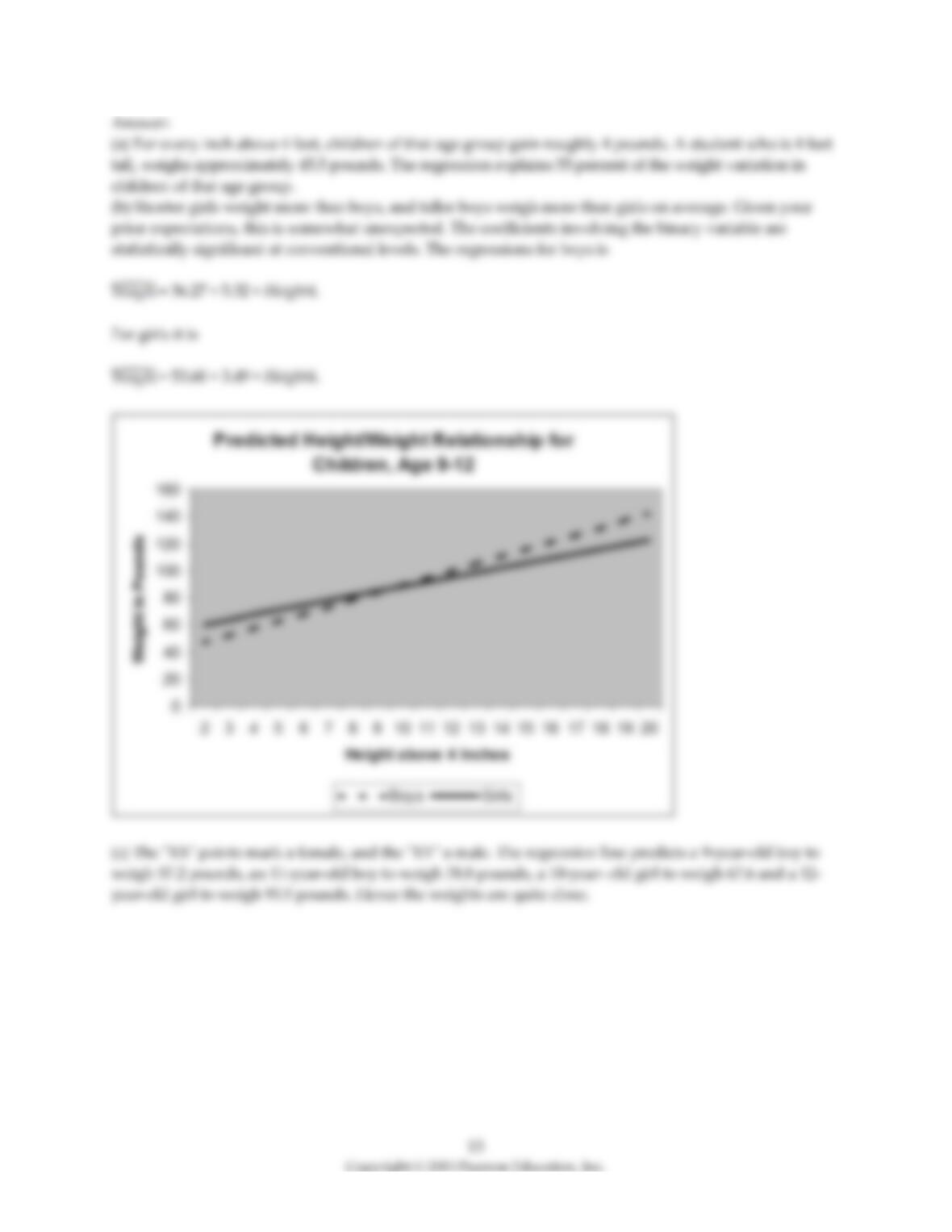
(b) You remember from the medical literature that females in the adult population are, on average,
shorter than males and weigh less. You also seem to have heard that females, controlling for height, are
supposed to weigh less than males. To see if this relationship holds for children, you add a binary
variable (DFY) that takes on the value one for girls and is zero otherwise. You estimate the following
regression function:
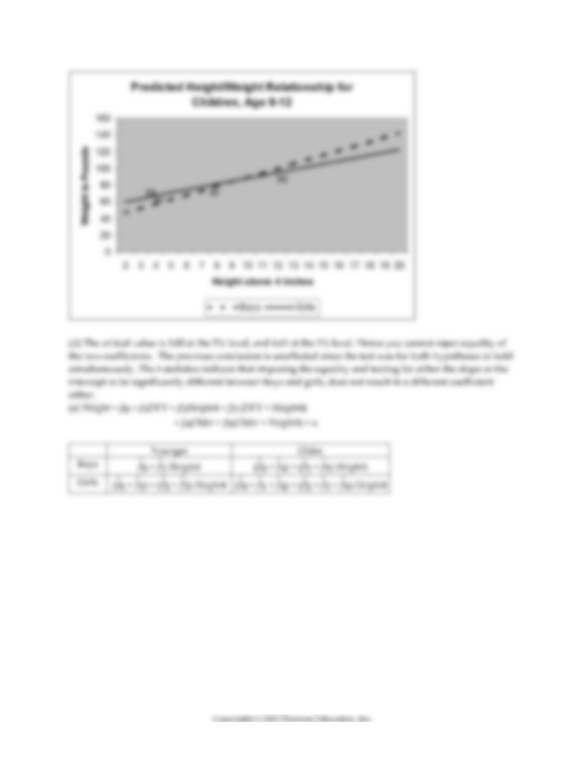
= 36.27 + 17.33 × DFY + 5.32 × Height4 – 1.83 × (DFY × Height4),
(5.99) (7.36) (0.80) (0.90)
R2 = 0.58, SER = 15.41
Are the signs on the new coefficients as expected? Are the new coefficients individually statistically
significant? Write down and sketch the regression function for boys and girls separately.
(c) The medical literature provides you with the following information for median height and weight of
nine- to twelve-year-olds:
Median Height and Weight for Children, Age 9-12
Boys’ Weight
Boys’ Height
Girls’ Weight
Girls’ Height
9-year-old
60
52
60
49
10-year-old
70
54
70
52
11-year-old
77
56
80
57
12-year-old
87
58.5
92
60
Insert two height/weight measures each for boys and girls and see how accurate your predictions are.
(d) The F-statistic for testing that the intercept and slope for boys and girls are identical is 2.92. Find the
critical values at the 5% and 1% level, and make a decision. Allowing for a different intercept with an
identical slope results in a t-statistic for DFY of (–0.35). Having identical intercepts but different slopes
gives a t-statistic on (DFYHeight4) of (–0.35) also. Does this affect your previous conclusion?
(e) Assume that you also wanted to test if the relationship changes by age. Briefly outline how you would
specify the regression including the gender binary variable and an age binary variable (Older) that takes
on a value of one for eleven to twelve year olds and is zero otherwise. Indicate in a table of two rows and
two columns how the estimated relationship would vary between younger girls, older girls, younger
boys, and older boys.
14
15
4) You have learned that earnings functions are one of the most investigated relationships in economics.
These typically relate the logarithm of earnings to a series of explanatory variables such as education,
work experience, gender, race, etc.
(a) Why do you think that researchers have preferred a log-linear specification over a linear specification?
In addition to the interpretation of the slope coefficients, also think about the distribution of the error
term.
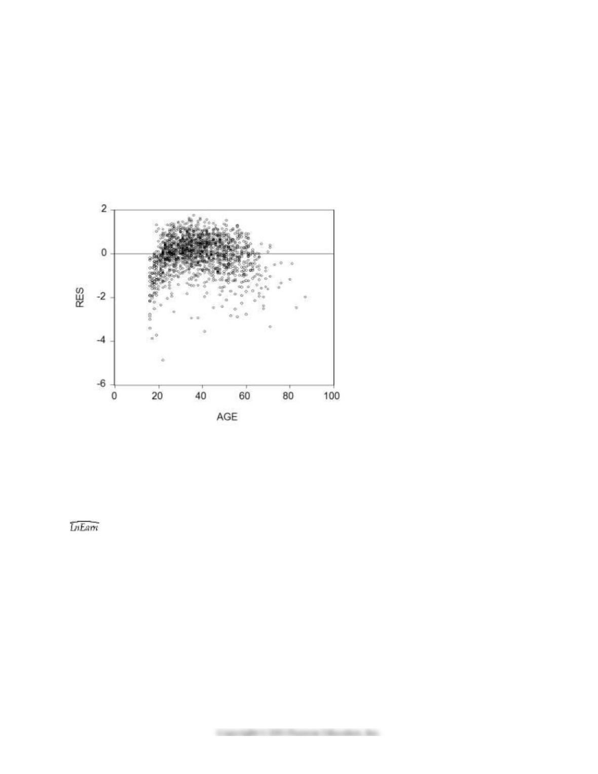
(b) To establish age-earnings profiles, you regress ln(Earn) on Age, where Earn is weekly earnings in
dollars, and Age is in years. Plotting the residuals of the regression against age for 1,744 individuals looks
as shown in the figure:
Do you sense a problem?
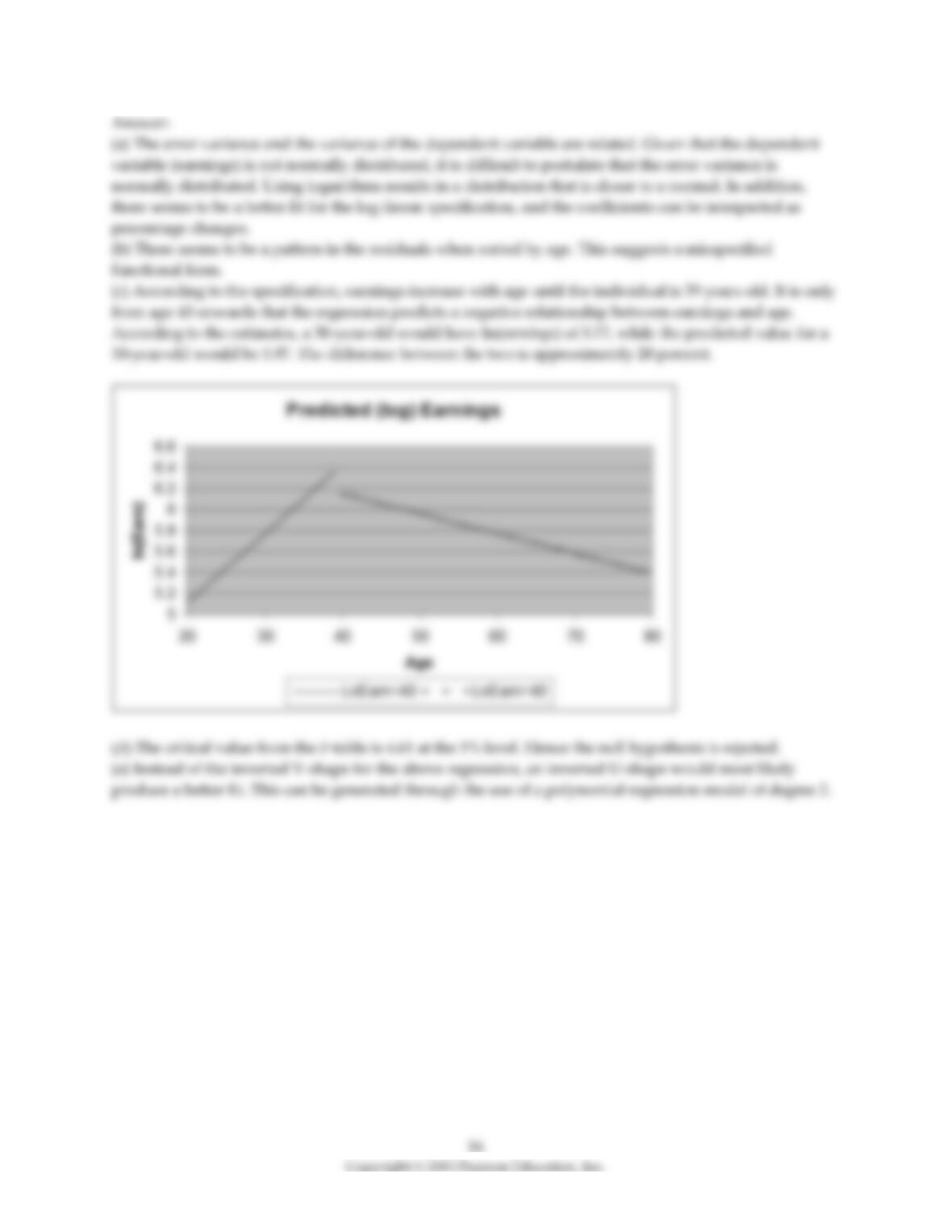
(c) You decide, given your knowledge of age-earning profiles, to allow the regression line to differ for the
below and above 40 years age category. Accordingly you create a binary variable, Dage, that takes the
value one for age 39 and below, and is zero otherwise. Estimating the earnings equation results in the
following output (using heteroskedasticity-robust standard errors):
= 6.92 – 3.13 × Dage – 0.019 × Age + 0.085 × (Dage × Age), R2=0.20, SER =0.721.
(38.33) (0.22) (0.004) (0.005)
Sketch both regression lines: one for the age category 39 years and under, and one for 40 and above. Does
it make sense to have a negative sign on the Age coefficient? Predict the ln(earnings) for a 30 year old and
a 50 year old. What is the percentage difference between these two?
(d) The F-statistic for the hypothesis that both slopes and intercepts are the same is 124.43. Can you reject
the null hypothesis?
(e) What other functional forms should you consider?

17
5) Sports economics typically looks at winning percentages of sports teams as one of various outputs, and
estimates production functions by analyzing the relationship between the winning percentage and
inputs. In Major League Baseball (MLB), the determinants of winning are quality pitching and batting.
All 30 MLB teams for the 1999 season. Pitching quality is approximated by “Team Earned Run Average”
(ERA), and hitting quality by “On Base Plus Slugging Percentage” (OPS).
Summary of the Distribution of Winning Percentage, On Base Plus Slugging Percentage,
and Team Earned Run Average for MLB in 1999
Average
Standard
deviation
Percentile
10%
25%
40%
50%
(median)
60%
75%
90%
Team ERA
4.71
0.53
3.84
4.35
4.72
4.78
4.91
5.06
5.25
OPS
0.778
0.034
0.720
0.754
0.769
0.780
0.790
0.798
0.820
Winning
Percentage
0.50
0.08
0.40
0.43
0.46
0.48
0.49
0.59
0.60
Your regression output is:
= –0.19 – 0.099 × teamera + 1.490 × ops, R2=0.92, SER = 0.02.
(0.08) (0.008) (0.126)
(a) Interpret the regression. Are the results statistically significant and important?
(b) There are two leagues in MLB, the American League (AL) and the National League (NL). One major
difference is that the pitcher in the AL does not have to bat. Instead there is a “designated hitter” in the
hitting line-up. You are concerned that, as a result, there is a different effect of pitching and hitting in the
AL from the NL. To test this hypothesis, you allow the AL regression to have a different intercept and
different slopes from the NL regression. You therefore create a binary variable for the American League
(DAL) and estimate the following specification:
= – 0.29 + 0.10 × DAL – 0.100 × teamera + 0.008 × (DAL× teamera)
(0.12) (0.24) (0.008) (0.018)
+ 1.622*ops – 0.187 *(DAL× ops) , R2=0.92, SER = 0.02.
(0.163) (0.160)
What is the regression for winning percentage in the AL and NL? Next, calculate the t-statistics and say
something about the statistical significance of the AL variables. Since you have allowed all slopes and the
intercept to vary between the two leagues, what would the results imply if all coefficients involving DAL
were statistically significant?
(c) You remember that sequentially testing the significance of slope coefficients is not the same as testing
for their significance simultaneously. Hence you ask your regression package to calculate the F-statistic
that all three coefficients involving the binary variable for the AL are zero. Your regression package gives
a value of 0.35. Looking at the critical value from you F-table, can you reject the null hypothesis at the 1%
level? Should you worry about the small sample size?

19
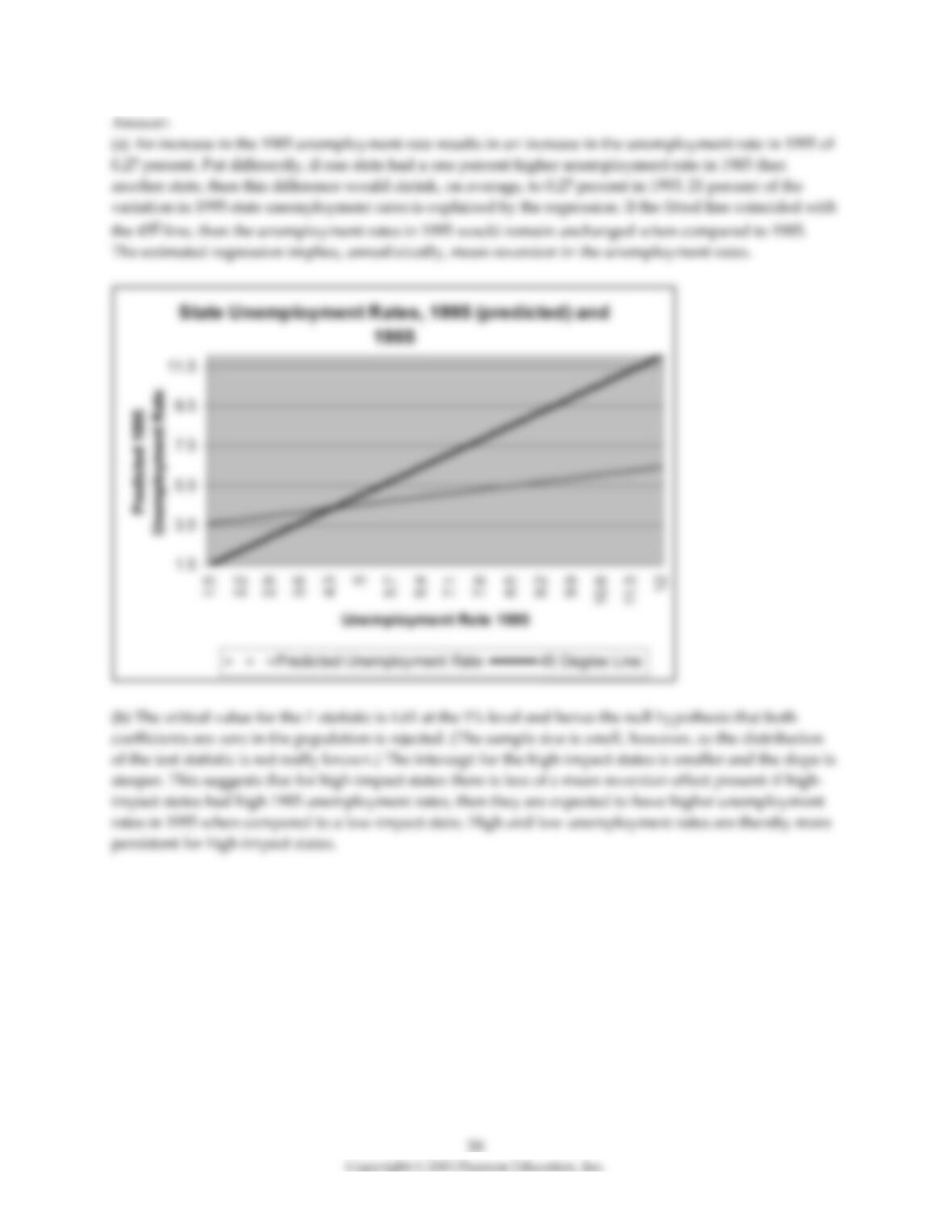
6) There has been much debate about the impact of minimum wages on employment and unemployment.
While most of the focus has been on the employment-to-population ratio of teenagers, you decide to
check if aggregate state unemployment rates have been affected. Your idea is to see if state
unemployment rates for the 48 contiguous U.S. states in 1985 can predict the unemployment rate for the
same states in 1995, and if this prediction can be improved upon by entering a binary variable for “high
impact” minimum wage states. One labor economist labeled states as high impact if a large fraction of
teenagers was affected by the 1990 and 1991 federal minimum wage increases. Your first regression
results in the following output:
= 3.19 + 0.27 × , R2 = 0.21, SER = 1.031
(0.56) (0.07)
(a) Sketch the regression line and add a 450 line to the graph. Interpret the regression results. What would
the interpretation be if the fitted line coincided with the 450 line?
(b) Adding the binary variable DhiImpact by allowing the slope and intercept to differ, results in the
following fitted line:
= 4.02 + 0.16 × – 3.25 × DhiImpact + 0.38 × (DhiImpact×),
(0.66) (0.09) (0.89) (0.11)
R2 = 0.31, SER=0.987
The F-statistic for the null hypothesis that both parameters involving the high impact minimum wage
variable are zero, is 42.16. Can you reject the null hypothesis that both coefficients are zero? Sketch the
two regression lines together with the 450 line and interpret the results again.
(c) To check the robustness of these results, you repeat the exercise using a new binary variable for the so-
called mining state (Dmining), i.e., the eleven states that have at least three percent of their total state
earnings derived from oil, gas extraction, and coal mining, in the 1980s. This results in the following
output:
= 4.04 + 0.15× – 2.92 × Dmining + 0.37 × (Dmining × ),
(0.65) (0.09) (0.90) (0.10)
R2 = 0.31, SER=0.997
How confident are you that the previously found effect is due to minimum wages?