21

22
7) Labor economists have extensively researched the determinants of earnings. Investment in human
capital, measured in years of education, and on the job training are some of the most important
explanatory variables in this research. You decide to apply earnings functions to the field of sports
economics by finding the determinants for baseball pitcher salaries. You collect data on 455 pitchers for
the 1998 baseball season and estimate the following equation using OLS and heteroskedasticity-robust
standard errors:
= 12.45 + 0.052 × Years + 0.00089 × Innings + 0.0032 × Saves
(0.08) (0.026) (0.00020) (0.0018)
– 0.0085 × ERA, R2 = 0.45, SER = 0.874
(0.0168)
where Earn is annual salary in dollars, Years is number of years in the major leagues, Innings is number of
innings pitched during the career before the 1998 season, Saves is number of saves during the career
before the 1998 season, and ERA is the earned run average before the 1998 season.
(a) What happens to earnings when the pitcher stays in the league for one additional year? Compare the
salaries of two relievers, one with 10 more saves than the other. What effect does pitching 100 more
innings have on the salary of the pitcher? What effect does reducing his ERA by 1.5? Do the signs
correspond to your expectations? Explain.
(b) Are the individual coefficients statistically significant? Indicate the level of significance you used and
the type of alternative hypothesis you considered.
(c) Although you are quite impressed with the fit of the regression, someone suggests that you should
include the square of years and innings as additional explanatory variables. Your results change as
follows:
= 12.15 + 0.160 × Years + 0.00268 × Innings + 0.0063 × Saves
(0.05) (0.039) (0.00030) (0.0010)
– 0.0584 × ERA – 0.0165 × Years2 – 0.00000045 × Innings2
(0.0165) (0.0026) (0.00000012)
R2 = 0.69, SER = 0.666
What is her reasoning? Are the coefficients of the quadratic terms statistically significant? Are they
meaningful?
(d) Calculate the effect of moving from two to three years, as opposed to from 12 to 13 years.
(e) You also decide to test the specification for stability across leagues (National League and American
League) by including a dummy variable for the National League and allowing the intercept and all slopes
to differ. The resulting F-statistic for restricting all coefficients that involve the National League dummy
variable to zero, is 0.40. Compare this to the relevant critical value from the table and decide whether or
not these additional variables should be included.

24
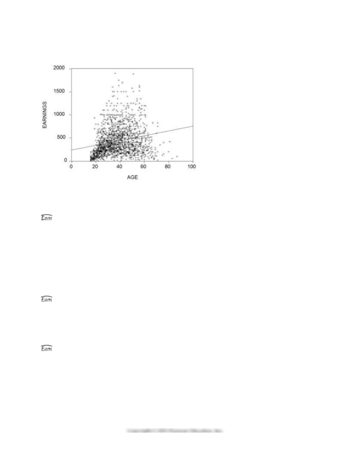
8) After analyzing the age-earnings profile for 1,744 workers as shown in the figure, it becomes clear to
you that the relationship cannot be approximately linear.
You estimate the following polynomial regression model, controlling for the effect of gender by using a
binary variable that takes on the value of one for females and is zero otherwise:
= –795.90 + 82.93 × Age – 1.69 × Age2 + 0.015 × Age3 – 0.0005 × Age4
(283.11) (29.29) (1.06) (0.016) (0.0009)
– 163.19 Female, R2=0.225, SER=259.78
(12.45)
(a) Test for the significance of the Age4 coefficient. Describe the general strategy to determine the
appropriate degree of the polynomial.
(b) You run two further regressions. Present an argument as to which one you should use for further
analysis.
= – 683.21 + 65.83 × Age – 1.05 × Age2 + 0.005 × Age3
120.13) (9.27) (0.22) (0.002)
– 163.23 Female, R2=0.225, SER=259.73
(12.45)
= – 344.88 + 41.48 × Age – 0.45× Age2
(51.58) (2.64) (0.03)
– 163.81 Female, R2=0.222, SER=260.22
(12.47)
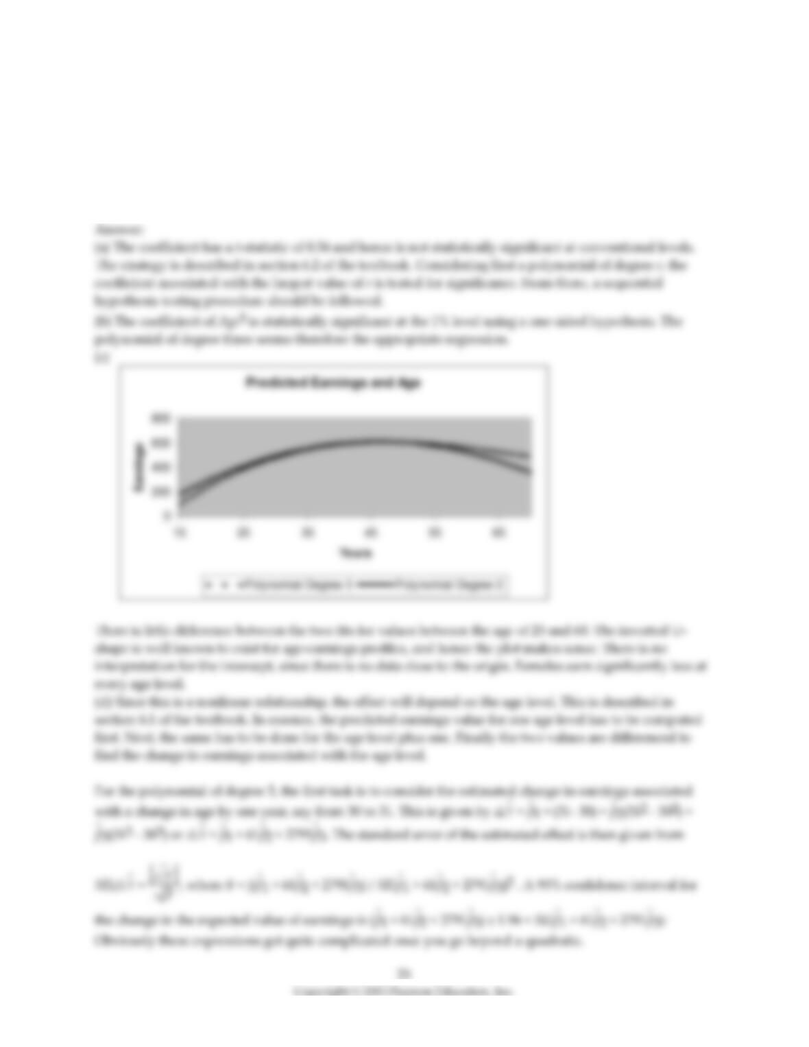
(c) Sketch the graph of fitted earnings of males against age of your preferred regression. Does this make
sense? Are you concerned about the negative coefficient on the regression intercept? What is the
implication for female earners in this sample?
(d) Explain how you would calculate the effect of changing age by one year on earnings, holding constant
the gender variable. Finally, briefly describe how you would calculate the standard errors of the
estimated effect.

26
9) Earnings functions attempt to find the determinants of earnings, using both continuous and binary
variables. One of the central questions analyzed in this relationship is the returns to education.
(a) Collecting data from 253 individuals, you estimate the following relationship
= 0.54 + 0.083 × Educ, R2 = 0.20, SER = 0.445
(0.14) (0.011)
where Earn is average hourly earnings and Educ is years of education.
What is the effect of an additional year of schooling? If you had a strong belief that years of high school
education were different from college education, how would you modify the equation? What if your
theory suggested that there was a “diploma effect”?
(b) You read in the literature that there should also be returns to on-the-job training. To approximate on-
the-job training, researchers often use the so called Mincer or potential experience variable, which is
defined as Exper = Age – Educ – 6. Explain the reasoning behind this approximation. Is it likely to
resemble years of employment for various sub-groups of the labor force?
(c) You incorporate the experience variable into your original regression
= -0.01 + 0.101 × Educ + 0.033 × Exper – 0.0005 × Exper2,
(0.16) (0.012) (0.006) (0.0001)
R2 = 0.34, SER = 0.405
What is the effect of an additional year of experience for a person who is 40 years old and had 12 years of
education? What about for a person who is 60 years old with the same education background?
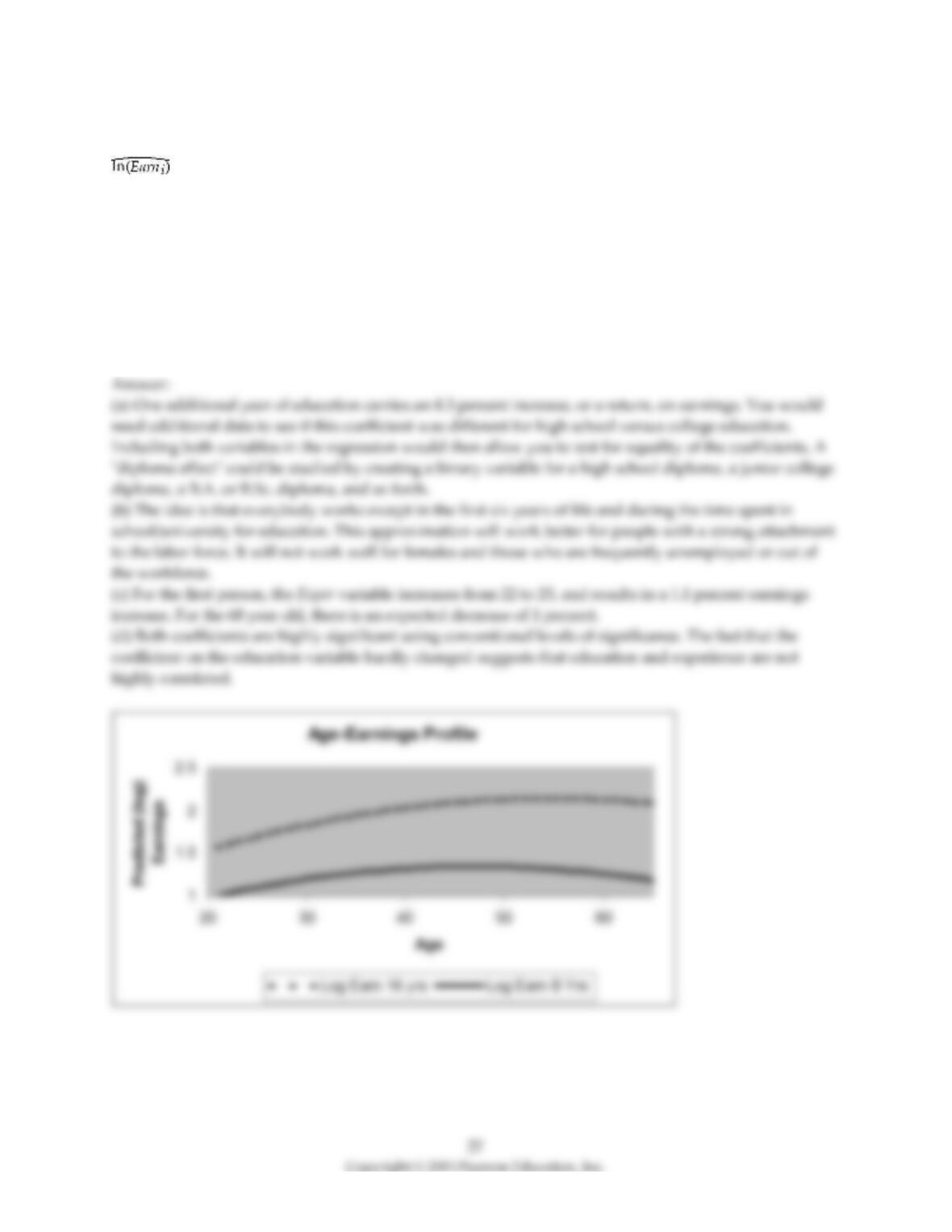
(d) Test for the significance of each of the coefficients of the added variables. Why has the coefficient on
education changed so little? Sketch the age-(log)earnings profile for workers with 8 years of education
and 16 years of education.
(e) You want to find the effect of introducing two variables, gender and marital status. Accordingly you
specify a binary variable that takes on the value of one for females and is zero otherwise (Female), and
another binary variable that is one if the worker is married but is zero otherwise (Married). Adding these
variables to the regressors results in:
= 0.21 + 0.093 × Educ + 0.032 × Exper – 0.0005 × Exper2
(0.16) (0.012) (0.006) (0.0001)
– 0.289 × Female + 0.062 Married,
(0.049) (0.056)
R2 = 0.43, SER = 0.378
Are the coefficients of the two added binary variables individually statistically significant? Are they
economically important? In percentage terms, how much less do females earn per hour, controlling for
education and experience? How much more do married people make? What is the percentage difference
in earnings between a single male and a married female? What is the marriage differential between males
and females?
(f) In your final specification, you allow for the binary variables to interact. The results are as follows:
= 0.14 + 0.093 × Educ + 0.032 × Exper – 0.0005 × Exper2
(0.16) (0.011) (0.006) (0.001)
– 0.158 × Female + 0.173 × Married – 0.218 × (Female × Married),
(0.075) (0.080) (0.097)
R2 = 0.44, SER = 0.375
Repeat the exercise in (e) of calculating the various percentage differences between gender and marital
status.

28
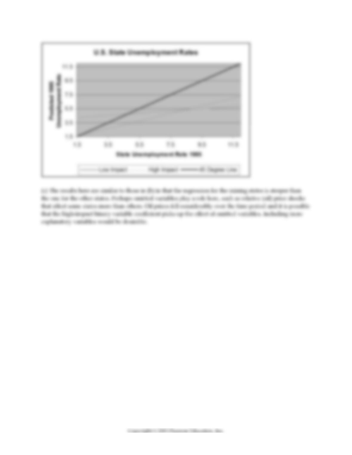
10) One of the most frequently estimated equations in the macroeconomics growth literature are so-called
convergence regressions. In essence the average per capita income growth rate is regressed on the
beginning-of-period per capita income level to see if countries that were further behind initially, grew
faster. Some macroeconomic models make this prediction, once other variables are controlled for. To
investigate this matter, you collect data from 104 countries for the sample period 1960-1990 and estimate
the following relationship (numbers in parentheses are for heteroskedasticity-robust standard errors):
= 0.020 – 0.360 × gpop + 0.00 4 × Educ – 0.053×RelProd60, R2=0.332, SER = 0.013
(0.009) (0.241) (0.001) (0.009)
where g6090 is the growth rate of GDP per worker for the 1960-1990 sample period, RelProd60 is the
initial starting level of GDP per worker relative to the United States in 1960, gpop is the average
population growth rate of the country, and Educ is educational attainment in years for 1985.
(a) What is the effect of an increase of 5 years in educational attainment? What would happen if a country
could implement policies to cut population growth by one percent? Are all coefficients significant at the
5% level? If one of the coefficients is not significant, should you automatically eliminate its variable from
the list of explanatory variables?
(b) The coefficient on the initial condition has to be significantly negative to suggest conditional
convergence. Furthermore, the larger this coefficient, in absolute terms, the faster the convergence will
take place. It has been suggested to you to interact education with the initial condition to test for
additional effects of education on growth. To test for this possibility, you estimate the following
regression:
= 0.015 – 0.323 × gpop + 0.005 × Educ – 0.051 × RelProd60
(0.009) (0.238) (0.001) (0.013)
–0.0028 × (EducRelProd60), R2=0.346, SER = 0.013
(0.0015)
Write down the effect of an additional year of education on growth. West Germany has a value for
RelProd60 of 0.57, while Brazil’s value is 0.23. What is the predicted growth rate effect of adding one year
of education in both countries? Does this predicted growth rate make sense?
(c) What is the implication for the speed of convergence? Is the interaction effect statistically significant?
(d) Convergence regressions are basically of the type
Δln Yt = β0 – β1 ln Y0
where
△
might be the change over a longer time period, 30 years, say, and the average growth rate is
used on the left-hand side. You note that the equation can be rewritten as
△ln Yt = β0 – (1 – β1) ln Y0
Over a century ago, Sir Francis Galton first coined the term “regression” by analyzing the relationship
between the height of children and the height of their parents. Estimating a function of the type above, he
found a positive intercept and a slope between zero and one. He therefore concluded that heights would
revert to the mean. Since ultimately this would imply the height of the population being the same, his
result has become known as “Galton’s Fallacy.” Your estimate of β1 above is approximately 0.05. Do you
see a parallel to Galton’s Fallacy?

11) Pages 283-284 in your textbook contain an analysis of the “Return to Education and the Gender Gap.”
Column (4) in Table 8.1 displays regression results using the 2009 Current Population Survey. The
equation below shows the regression result for the same specification, but using the 2005 Current
Population Survey. Interpret the major results.
= 1.215 + 0.0899 × educ – 0.521 × DFemme+ 0.0180 × (DFemme×educ)
(0.018) (0.0011) (0.022) (0.0016)
+ 0.0232 × exper – 0.000368 × exper2 – 0.058 × Midwest – 0.0098 × South – 0.030 × West
(0.0008) (0.000018) (0.006) (0.0078) (0.0030)
8.3 Mathematical and Graphical Problems
1) Give at least three examples from economics where you expect some nonlinearity in the relationship
between variables. Interpret the slope in each case.
2) Suggest a transformation in the variables that will linearize the deterministic part of the population
regression functions below. Write the resulting regression function in a form that can be estimated by
using OLS.
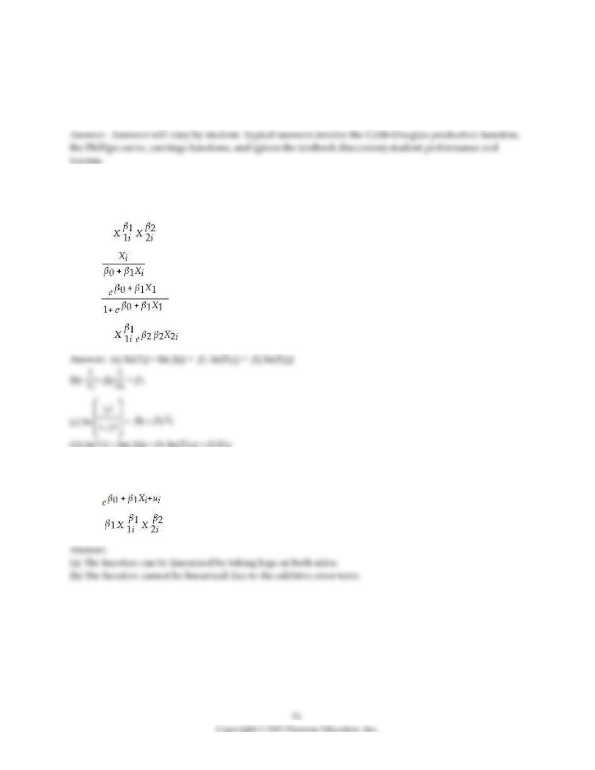
(a) Yi = β0
(b) Yi =
(c) Yi =
(d) Yi = β0
3) Indicate whether or not you can linearize the regression functions below so that OLS estimation
methods can be applied:
(a) Yi =
(b) Yi = + ui
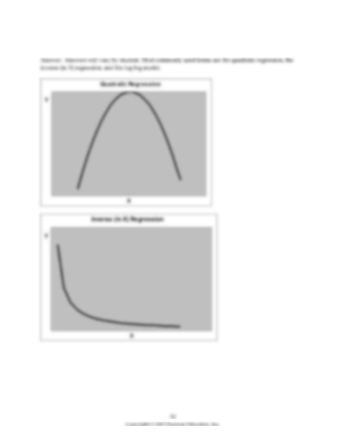
4) Choose at least three different nonlinear functional forms of a single independent variable and sketch
the relationship between the dependent and independent variable.