11) Using the 420 observations of the California School data set from your textbook, you estimate the
following relationship:
= 681.44 – 0.61LchPct
n=420, R2=0.75, SER=9.45
where TestScore is the test score and LchPct is the percent of students eligible for subsidized lunch
(average = 44.7, max = 100, min = 0).
a. Interpret the regression result.
b. In your interpretation of the slope coefficient in (a) above, does it matter if you start your explanation
with “for every x percent increase” rather than “for every x percentage point increase”?
c. The “overall” regression F–statistic is 1149.57. What are the degrees of freedom for this statistic?
d. Find the critical value of the F–statistic at the 1% significance level. Test the null hypothesis that the
regression R2= 0.
e. The above equation was estimated using heteroskedasticity robust standard errors. What is the
standard error for the slope coefficient?
12) Consider the following regression using the California School data set from your textbook.
= 681.44 – 0.61LchPct
n=420, R2=0.75, SER=9.45
where TestScore is the test score and LchPct is the percent of students eligible for subsidized lunch
(average = 44.7, max = 100, min = 0).
a. What is the effect of a 20 percentage point increase in the student eligible for subsidized lunch?
b. Your textbook started with the following regression in Chapter 4:
= 698.9 – 2.28STR
n=420, R2=0.051, SER=18.58
where STR is the student teacher ratio.
Your textbook tells you that in the multiple regression framework considered, the percentage of students
eligible for subsidized lunch is a control variable, while the student teacher ratio is the variable of interest.
Given that the regression R2 is so much higher for the first equation than for the second equation,
shouldn’t the role of the two variables be reversed? That is, shouldn’t the student teacher ratio be the
control variable while the percent of students eligible for subsidized lunch be the variable of interest?
7.3 Mathematical and Graphical Problems
1) Explain carefully why testing joint hypotheses simultaneously, using the F–statistic, does not
necessarily yield the same conclusion as testing them sequentially (“one at a time” method), using a series
of t–statistics.
2) Set up the null hypothesis and alternative hypothesis carefully for the following cases:
(a) k = 4, test for all coefficients other than the intercept to be zero
(b) k = 3, test for the slope coefficient of X1 to be unity, and the coefficients on the other explanatory
variables to be zero
(c) k = 10, test for the slope coefficient of X1 to be zero, and for the slope coefficients of X2 and X3 to be
the same but of opposite sign.
(d) k = 4, test for the slope coefficients to add up to unity
3) Consider a situation where economic theory suggests that you impose certain restrictions on your
estimated multiple regression function. These may involve the equality of parameters, such as the returns
to education and on the job training in earnings functions, or the sum of coefficients, such as constant
returns to scale in a production function. To test the validity of your restrictions, you have your statistical
package calculate the corresponding F–statistic. Find the critical value from the F–distribution at the 5%
and 1% level, and comment whether or not you will reject the null hypothesis in each of the following
cases.
(a) number of observations: 152; number of restrictions: 3; F–statistic: 3.21
(b) number of observations: 1,732; number of restrictions:7; F–statistic: 4.92
(c) number of observations: 63; number of restrictions: 1; F–statistic: 2.47
(d) number of observations: 4,000; number of restrictions: 5; F–statistic: 1.82
(e) Explain why you can use the Fq,∞ distribution to compute the critical values in (a)–(d).
4) Females, on average, are shorter and weigh less than males. One of your friends, who is a pre–med
student, tells you that in addition, females will weigh less for a given height. To test this hypothesis, you
collect height and weight of 29 female and 81 male students at your university. A regression of the weight
on a constant, height, and a binary variable, which takes a value of one for females and is zero otherwise,
yields the following result:
= –229.21 – 6.36 × Female + 5.58 × Height, R2=0.50, SER = 20.99
(43.39) (5.74) (0.62)
where Studentw is weight measured in pounds and Height is measured in inches (heteroskedasticity–
robust standard errors in parentheses).
Calculate t–statistics and carry out the hypothesis test that females weigh the same as males, on average,
for a given height, using a 10% significance level. What is the alternative hypothesis? What is the p–value?
What critical value did you use?
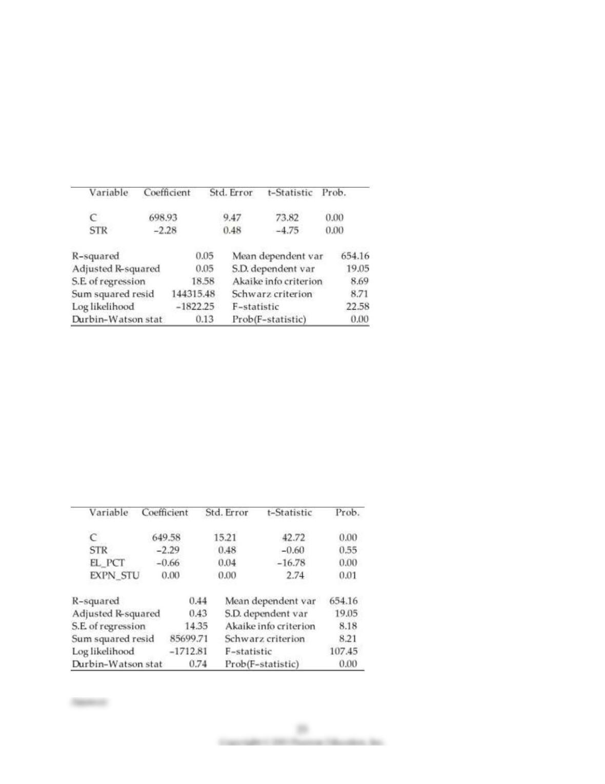
5) You are presented with the following output from a regression package, which reproduces the
regression results of testscores on the student–teacher ratio from your textbook
Dependent Variable: TESTSCR
Method: Least Squares
Date: 07/30/06 Time: 17:44
Sample: 1 420
Included observations: 420
Std. Error are homoskedasticity only standard errors.
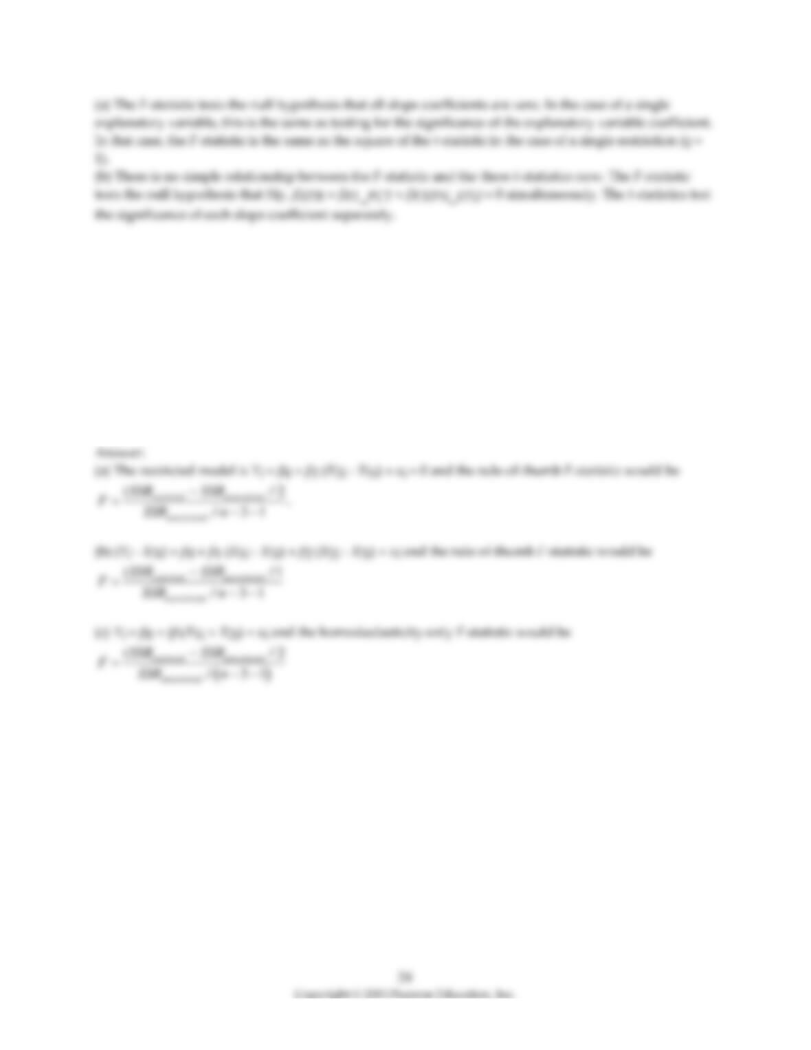
a) What is the relationship between the t–statistic on the student–teacher ratio coefficient and the F–
statistic?
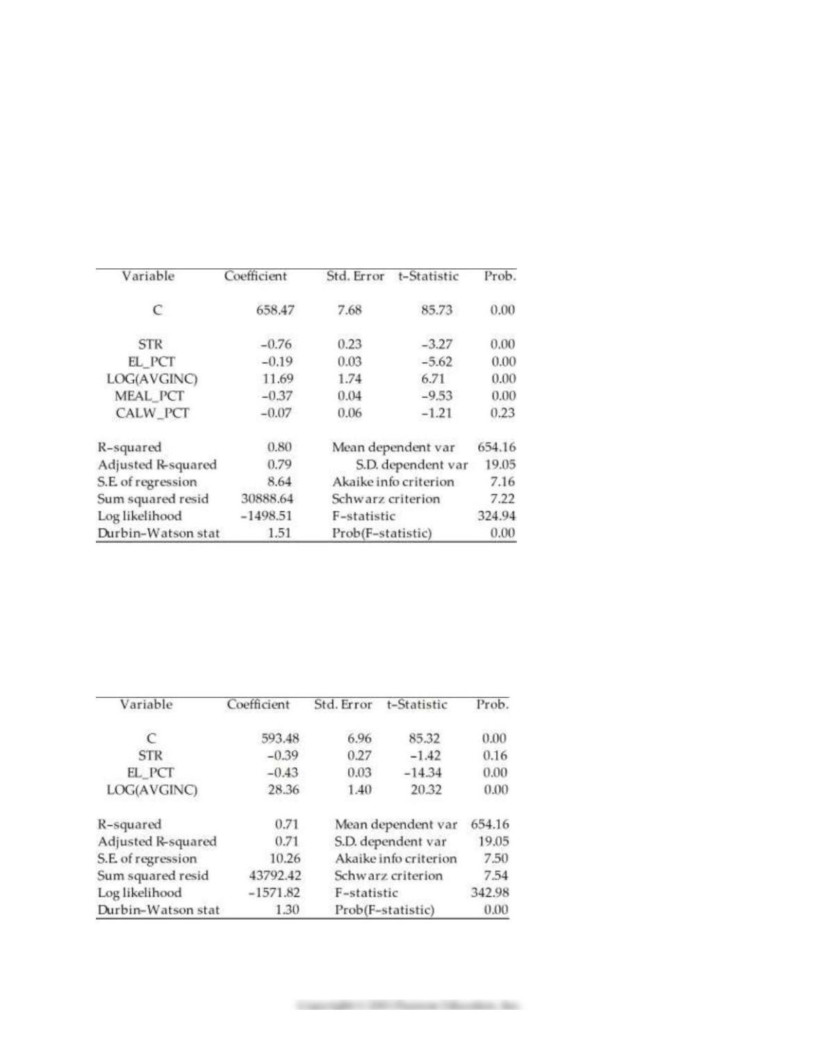
b) Next, two explanatory variables, the percent of English learners (EL_PCT) and expenditures per
student (EXPN_STU) are added. The output is listed as below. What is the relationship between the three
t–statistics for the slopes and the homoskedasticity–only F–statistic now?
Dependent Variable: TESTSCR
Method: Least Squares
Date: 07/30/06 Time: 17:55
Sample: 1 420
Included observations: 420
6) Consider the following multiple regression model
Yi = β0 + β1X1i + β2X2i + β3X3i + ui
You want to consider certain hypotheses involving more than one parameter, and you know that the
regression error is homoskedastic. You decide to test the joint hypotheses using the homoskedasticity–
only F–statistics. For each of the cases below specify a restricted model and indicate how you would
compute the F–statistic to test for the validity of the restrictions.
(a) β1 = –β2; β3 = 0
(b) β1 + β2 + β3 = 1
(c) β1 = β2; β3 = 0
7) Give an intuitive explanation for
( )
(/
/1
restricted unrestricted
unrestricted unrestriced
SSR SSR q
FSSR n k
−
=−−
. Name conditions under which
the F–statistic is large and hence rejects the null hypothesis.
8) Prove that
( ) ( )
22
2
( / /
/ 1 1 / 1
restricted unrestricted unrestriced restriced
unrestricted unrestriced unrestriced unrestriced
SSR SSR q R R q
FSSR n k R n k
−−
==
− − − − −

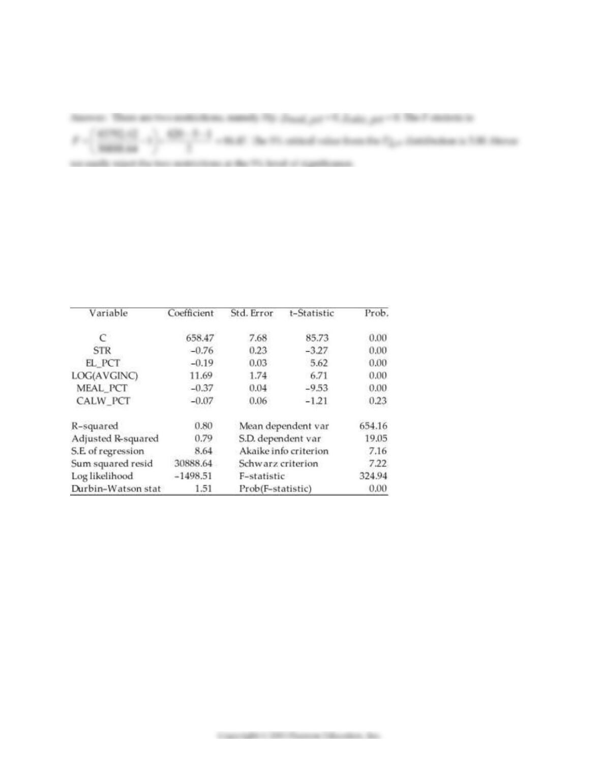
9) To calculate the homoskedasticity–only overall regression F–statistic, you need to compare the
SSRrestricted with the SSRunrestricted. Consider the following output from a regression package, which
reproduces the regression results of testscores on the student–teacher ratio, the percent of English
learners, and the expenditures per student from your textbook:
Dependent Variable: TESTSCR
Method: Least Squares
Date: 07/30/06 Time: 17:55
Sample: 1 420
Included observations: 420
Sum of squared resid corresponds to SSRunrestricted. How are you going to find SSRrestricted?
10) Adding the Percent of English Speakers (PctEL) to the Student Teacher Ratio (STR) in your textbook
reduced the coefficient for STR from 2.28 to 1.10 with a standard error of 0.43. Construct a 90% and 99%
confidence interval to test the hypothesis that the coefficient of STR is 2.28.
11) The homoskedasticity only F–statistic is given by the formula
( )
( ) /
/1
restricted unrestricted
unrestricted unrestriced
SSR SSR q
FSSR n k
−
=−−
where SSRrestricted is the sum of squared residuals from the restricted regression, SSRunrestricted is the
sum of squared residuals from the unrestricted regression, q is the number of restrictions under the null
hypothesis, and kunrestricted is the number of regressors in the unrestricted regression. Prove that this
formula is the same as the following formula based on the regression R2 of the restricted and unrestricted
regression:
( )
( ) /
1 / 1
restricted unrestricted
unrestricted unrestriced
ESS ESS q
FESS n k
−
=− − −
12) Trying to remember the formula for the homoskedasticity–only F–statistic, you forgot whether you
subtract the restricted SSR from the unrestricted SSR or the other way around. Your professor has
provided you with a table containing critical values for the F distribution. How can this be of help?
28
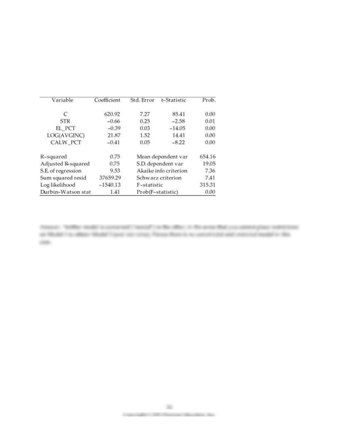
13) Consider the following regression output for an unrestricted and a restricted model.
Unrestricted model:
Dependent Variable: TESTSCR
Method: Least Squares
Date: 07/31/06 Time: 17:35
Sample: 1 420
Included observations: 420
Restricted model:
Dependent Variable: TESTSCR
Method: Least Squares
Date: 07/31/06 Time: 17:37
Sample: 1 420
Included observations: 420
29
Calculate the homoskedasticity only F–statistic and determine whether the null hypothesis can be rejected
at the 5% significance level.
14) Consider the regression output from the following unrestricted model:
Unrestricted model:
Dependent Variable: TESTSCR
Method: Least Squares
Date: 07/31/06 Time: 17:35
Sample: 1 420
Included observations: 420
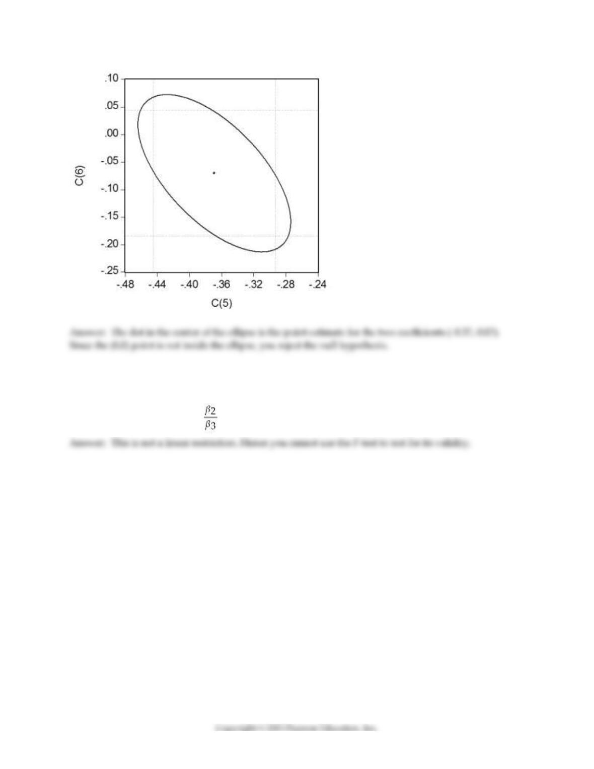
To test for the null hypothesis that neither coefficient on the percent eligible for subsidized lunch nor the
coefficient on the percent on public income assistance is statistically significant, you have your statistical
package plot the confidence set. Interpret the graph below and explain what it tells you about the null
hypothesis.
30
15) Consider the regression model Yi = β0 + β1X1i + β2X2i+ β3X3i + ui. Use “Approach #2” from Section
7.3 to transform the regression so that you can use a t–statistic to test:
β1 =
31
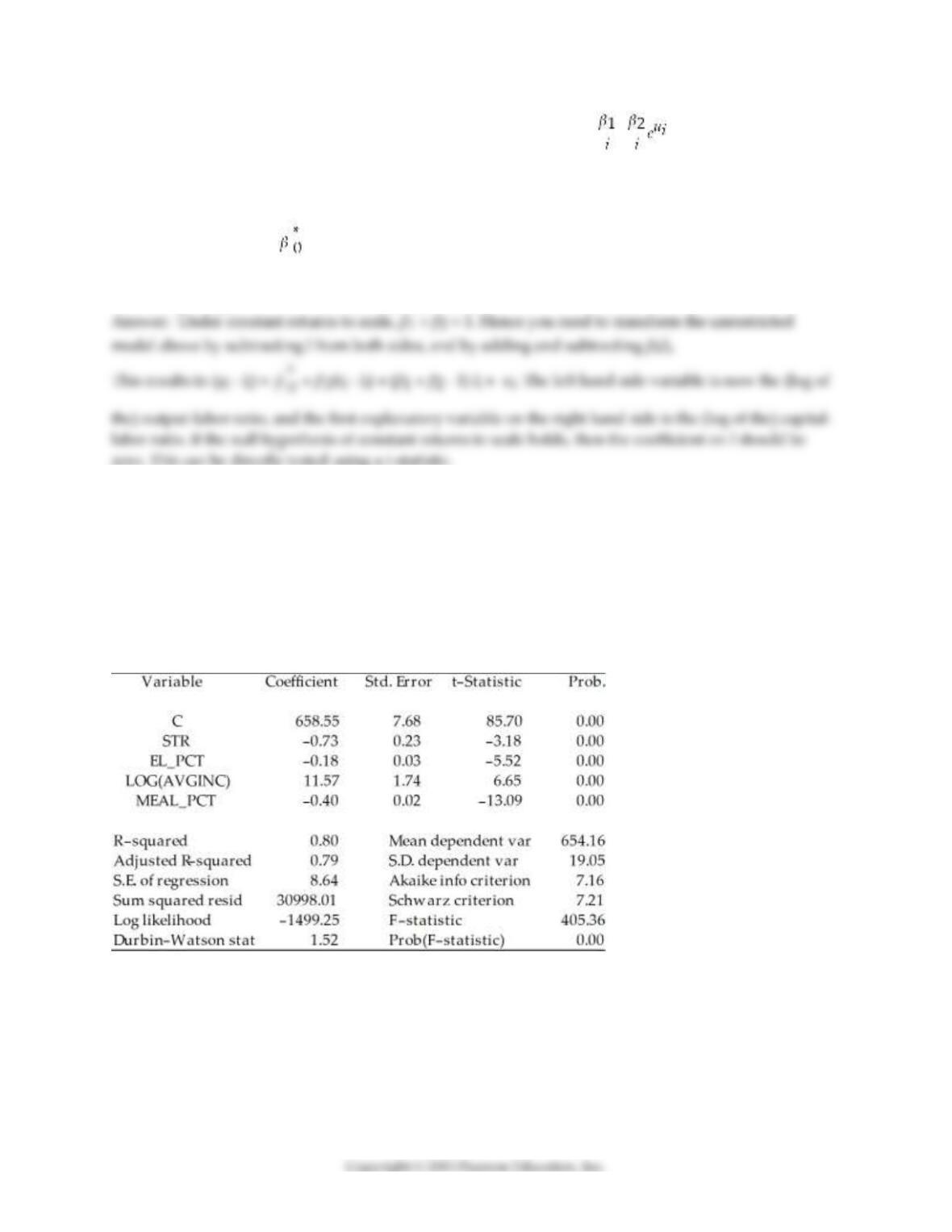
16) Consider the following Cobb–Douglas production function Yi = AK L (where Y is output, A is
the level of technology, K is the capital stock, and L is the labor force), which has been linearized here (by
using logarithms) to look as follows:
yi = + β1ki + β2li + ui
Assuming that the errors are heteroskedastic, you want to test for constant returns to scale. Using a t–
statistic and “Approach #2,” how would you proceed.
17) Consider the following two models to explain testscores.
Model 1:
Dependent Variable: TESTSCR
Method: Least Squares
Date: 07/31/06 Time: 17:52
Sample: 1 420
Included observations: 420
Model 2:
Dependent Variable: TESTSCR
Method: Least Squares
Date: 07/31/06 Time: 17:56
Sample: 1 420
Included observations: 420
Explain why you cannot use the F–test in this situation to discriminate between Model 1 and Model 2.
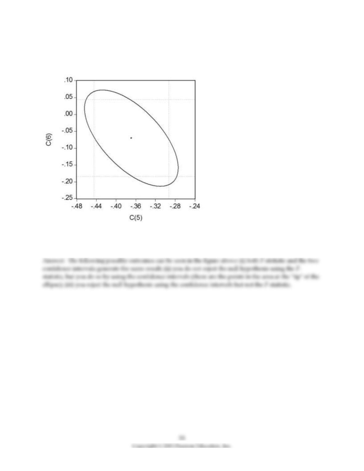
18) Your textbook has emphasized that testing two hypothesis sequentially is not the same as testing
them simultaneously. Consider the following confidence set below, where you are testing the hypothesis
that H0 : β5 = 0, β6 = 0.
Your statistical package has also generated a dotted area, which corresponds to drawing two confidence
intervals for the respective coefficients. For each case where the ellipse does not coincide in area with the
corresponding rectangle, indicate what your decision would be if you relied on the two confidence
intervals vs. the ellipse generated by the F–statistic.
19) You have estimated the following regression to explain hourly wages, using a sample of 250
individuals:
AHEi = –2.44 – 1.57 × DFemme + 0.27 × DMarried + 0.59 × Educ + 0.04 × Exper – 0.60 × DNonwhite
(1.29) (0.33) (0.36) (0.09) (0.01) (0.49)
+ 0.13 × NCentral – 0.11 × South
(0.59) (0.58)
R2 = 0.36, SER = 2.74, n = 250
Numbers in parenthesis are heteroskedasticity robust standard errors. Add “*”(5%) and “**” (1%) to
indicate statistical significance of the coefficients.
20) You have estimated the following regression to explain hourly wages, using a sample of 250
individuals:
= –2.44 – 1.57 × DFemme + 0.27 × DMarried + 0.59 × Educ + 0.04 × Exper – 0.60 × DNonwhite
(1.29) (0.33) (0.36) (0.09) (0.01) (0.49)
+ 0.13 × NCentral – 0.11 × South
(0.59) (0.58)
R2 = 0.36, SER = 2.74, n = 250
Test the null hypothesis that the coefficients on DMarried, DNonwhite, and the two regional variables,
NCentral and South are zero. The F–statistic for the null hypothesis βmarried = βnonwhite = βnonwhite =
βncentral = βsouth = 0 is 0.61. Do you reject the null hypothesis?
21) Using the California School data set from your textbook, you decide to run a regression of the average
reading score (ScrRead) on the average mathematics score (ScrMaths). The result is as follows, where the
numbers in parenthesis are homoskedasticity only standard errors:
= 8.47 + 0.9895×ScrMaths
(13.20) (0.0202)
N = 420, R2 = 0.85, SER = 7.8
You believe that the average mathematics score is an unbiased predictor of the average reading score.
Consider the above regression to be the unrestricted from which you would calculate SSRUnrestricted .
How would you find the SSRRestricted? How many restrictions would have to impose?
22) Looking at formula (7.13) in your textbook for the homoskedasticity–only F–statistic,
( )
( )
unrestricted
/
/1
restricted unrestriced
unrestricted
SSR SSR q
FSSR n k
−
=−−
give three conditions under which, ceteris paribus, you would find a large value, and hence would be
likely to reject the null hypothesis.
23) Analyzing a regression using data from a sub–sample of the Current Population Survey with about
4,000 observations, you realize that the regression R2, and the adjusted R2, 2, are almost identical. Why is
that the case? In your textbook, you were told that the regression R2 will almost always increase when
you add an explanatory variable, but that the adjusted measure does not have to increase with such an
addition. Can this still be true?