b.
decreasing returns to scale.
c.
constant returns to scale.
d.
increasing costs per unit of output.
DISC: Costs of production
United States – BPROG: Analytic
Costs of production
Economies of Scale
180. If a firm increases inputs by 15 percent and output increases by 12.5 percent, the firm is experiencing
a.
increasing returns to scale.
b.
decreasing returns to scale.
c.
constant returns to scale.
d.
increasing costs per unit of output.
DISC: Costs of production
United States – BPROG: Analytic
Costs of production
Economies of Scale
181. If in some range of production average cost is falling, the firm is experiencing
a.
increasing returns to scale.
b.
decreasing returns to scale.
c.
constant returns to scale.
d.
increasing costs per unit of output.
DISC: Costs of production
United States – BPROG: Analytic
Costs of production
Economies of Scale
182. If in some production range average cost is rising, the firm is experiencing
a.
increasing returns to scale.
b.
decreasing returns to scale.
c.
constant returns to scale.
d.
increasing costs per unit of output.
1
DISC: Costs of production
United States – BPROG: Analytic
Costs of production
Economies of Scale
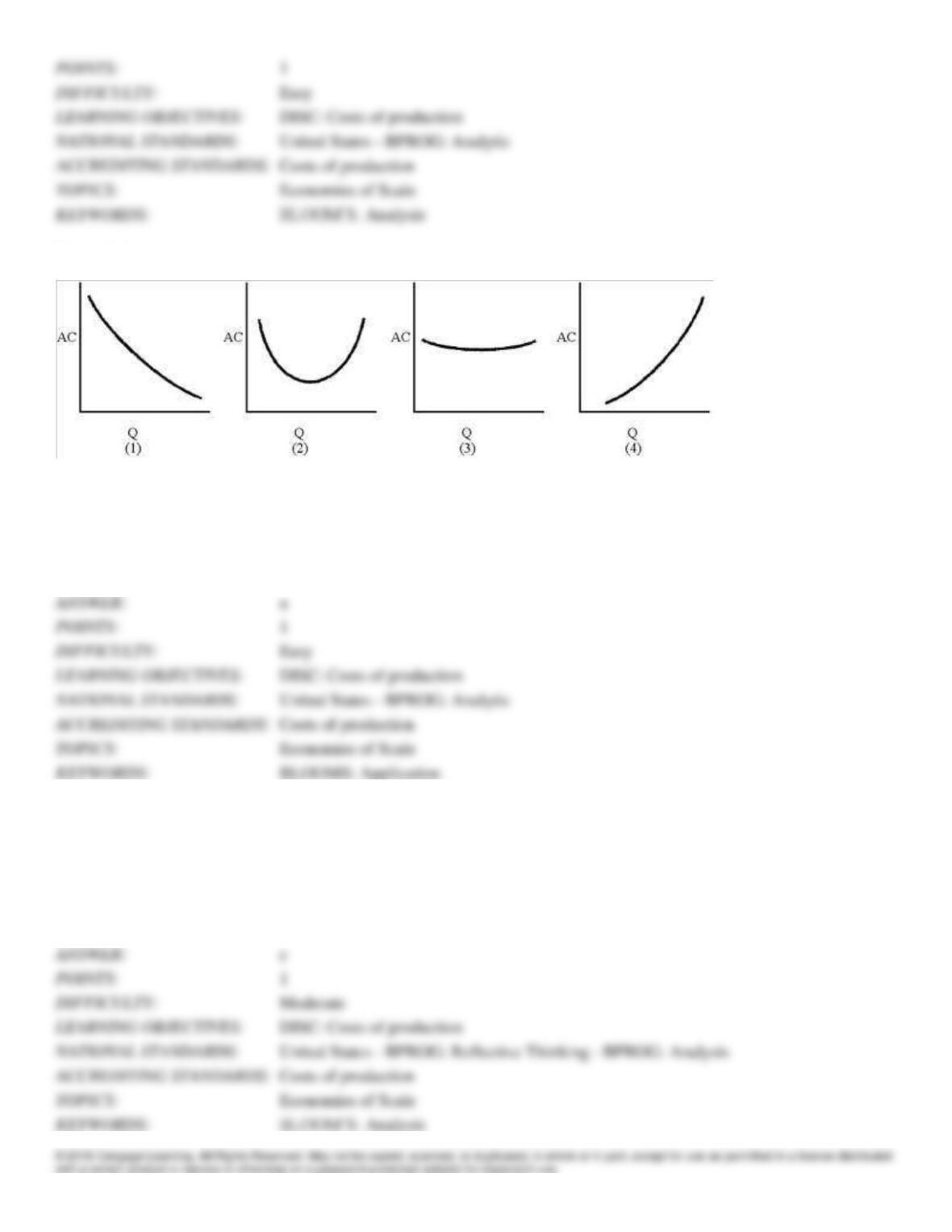
Figure 7-14
183. Of the long-run AC curves in Figure 7-14, which displays increasing returns to scale for all levels of output?
a.
1
b.
2
c.
3
d.
4
1
DISC: Costs of production
United States – BPROG: Analytic
Costs of production
Economies of Scale
BLOOMS: Application
184. A Detroit business advertises, “The more we sell, the lower the price, and the lower the price, the more we sell.” This
firm is experiencing
a.
decreasing returns to scale.
b.
constant returns to scale.
c.
increasing returns to scale.
d.
abnormal demand patterns.
1
DISC: Costs of production
United States – BPROG: Reflective Thinking – BPROG: Analysis
Economies of Scale
185. An airline industry study recently reported, “Evidence is abundant that larger firms are not more efficient or less
costly simply because they are larger. In fact, other things equal, the largest carriers tend to have a higher level of unit
costs, possibly caused by the difficulties of managing an airline of large size.” This means that
a.
there are increasing returns to scale in the airline industry.
b.
the airline industry has constant returns to scale.
c.
the larger airlines are not profitable.
d.
airlines are experiencing decreasing returns to scale.
DISC: Costs of production
United States – BPROG: Reflective Thinking – BPROG: Analysis
Costs of production
Economies of Scale
186. A cost curve drawn with years on the horizontal axis and costs per unit on the vertical axis would be a(n)
a.
analytical cost curve.
b.
long-run cost curve.
c.
historical cost curve.
d.
theoretical cost curve.
DISC: Costs of production
United States – BPROG: Analytic
Costs of production
Economies of Scale
187. Cost minimization is the process of making optimal use of all of the inputs whose quantities are
a.
set in the short run.
b.
set in the intermediate run.
c.
set in the long run.
d.
variable in the short and long run.
DISC: Costs of production
United States – BPROG: Analytic
Costs of production
Economies of Scale
188. The major incentive for cost minimization is the
a.
power of shareholders in the company.
b.
fear of top management by workers.
c.
discipline imposed by the market system.
d.
impact on U.S. corporations of taxing by the government.
DISC: Costs of production
United States – BPROG: Analytic
Costs of production
Economies of Scale
189. Production indifference curves bow inward toward the graph’s origin because of
a.
the law of diminishing returns to a single input.
b.
the law of diminishing marginal returns to scale.
c.
constant returns to scale.
d.
minimizing costs in the short run.
DISC: Costs of production
United States – BPROG: Analytic
Costs of production
190. Production costs for a given output will be minimized when the
a.
budget line and the product indifference curve meet in the vertical axis.
b.
budget line crosses the product indifference curve.
c.
budget line begins to bend back on itself.
d.
product indifference curve and the budget line are tangent.
DISC: Costs of production
United States – BPROG: Reflective Thinking – BPROG: Analysis
Costs of production
Characteristics of the Production Indifference Curves, or Isoquants
191. If on a given product indifference curve a firm is using an insufficient (nonoptimal) amount of one of its inputs
a.
output will be below optimal.
b.
the MRP of the input will be below its price.
c.
costs will not be minimal.
d.
relative input prices need to change.
DISC: Costs of production
United States – BPROG: Reflective Thinking – BPROG: Analysis
Costs of production
Characteristics of the Production Indifference Curves, or Isoquants
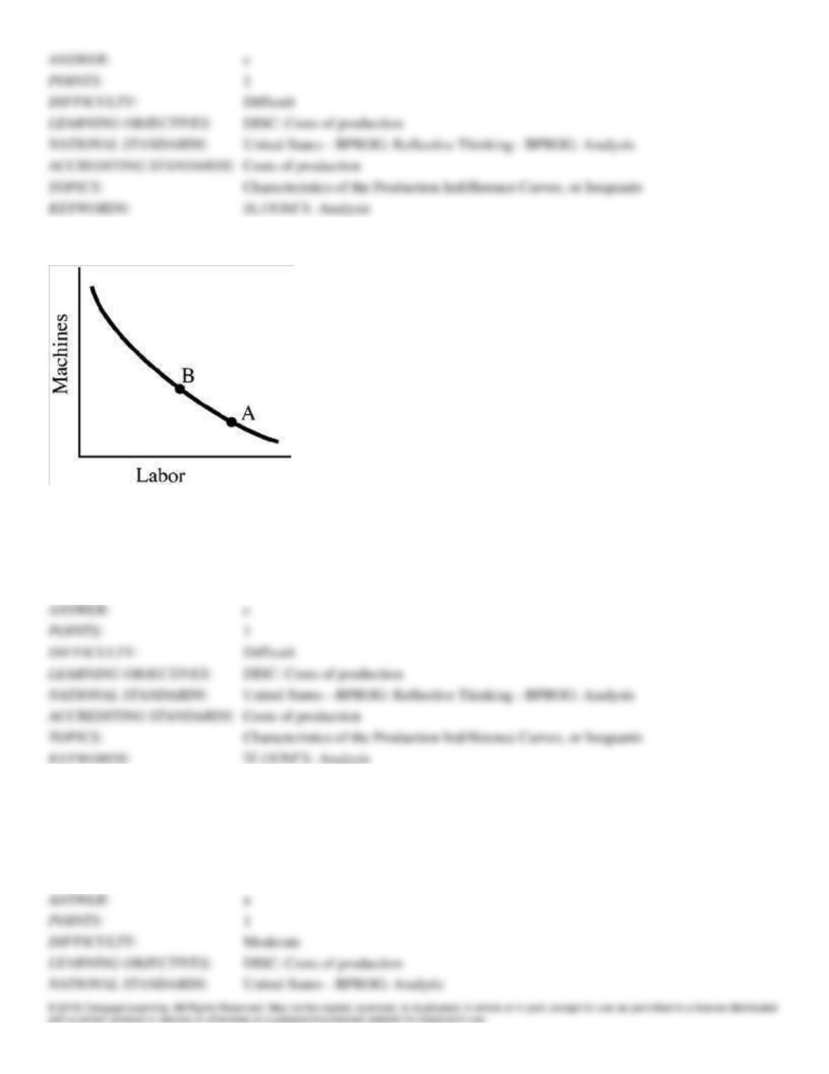
Figure 7-15
192. For a firm at equilibrium, at point A in Figure 7-15
a.
the price of labor is high relative to the price of machines.
b.
the MPP of labor is greater than the MPP of machines.
c.
the MPP of labor is less than at point B.
d.
output is higher than at point B.
DISC: Costs of production
United States – BPROG: Reflective Thinking – BPROG: Analysis
Costs of production
Characteristics of the Production Indifference Curves, or Isoquants
193. In Figure 7-15, we would expect a move of the budget line from A to B if
a.
the price of machines falls.
b.
the price of labor falls.
c.
output falls.
d.
the product price rises.
DISC: Costs of production
United States – BPROG: Analytic
Costs of production
Characteristics of the Production Indifference Curves, or Isoquants
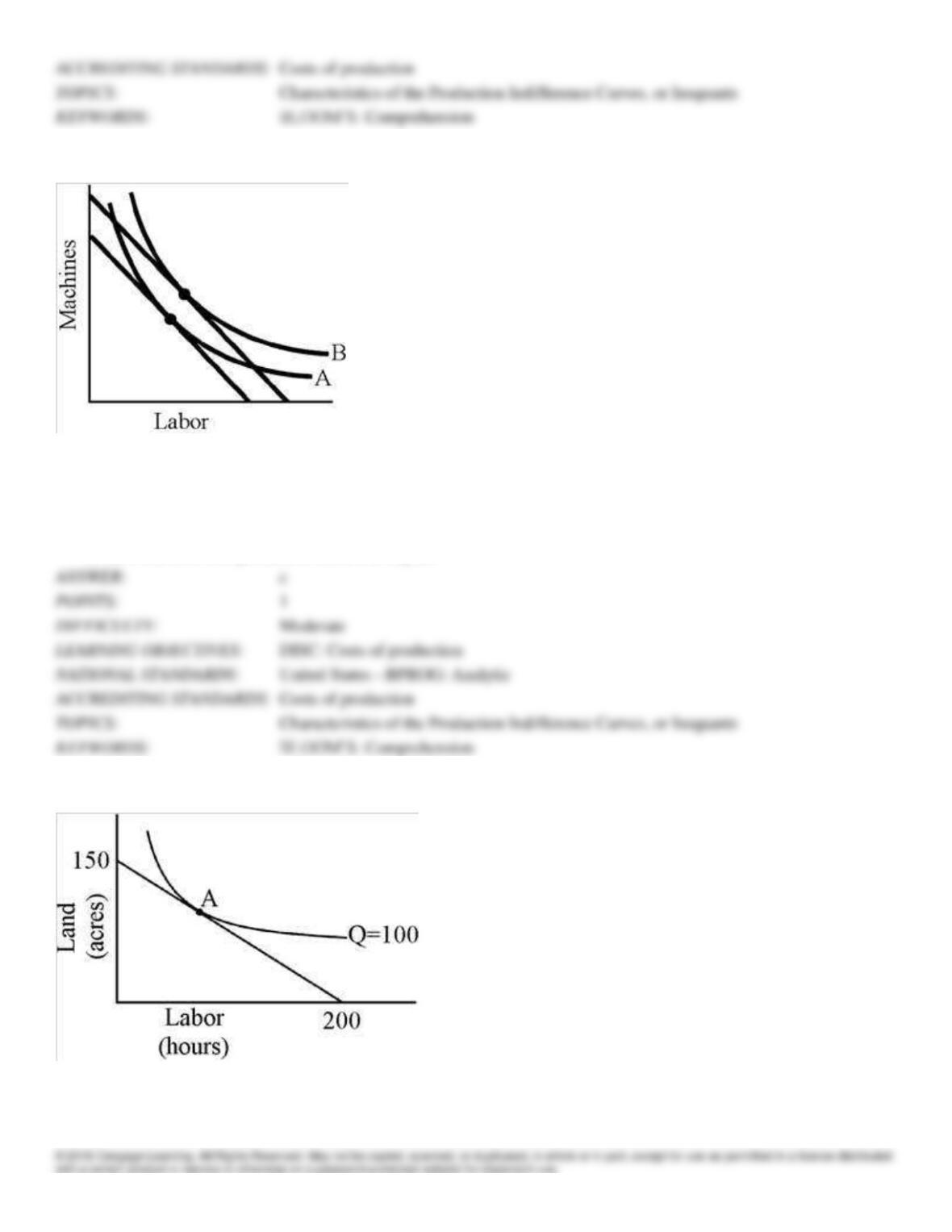
Figure 7-16
194. In Figure 7-16, as we move from A to B,
a.
the relative price of machines falls.
b.
total cost falls.
c.
output increases.
d.
labor becomes less productive relative to capital.
DISC: Costs of production
United States – BPROG: Analytic
Costs of production
Characteristics of the Production Indifference Curves, or Isoquants
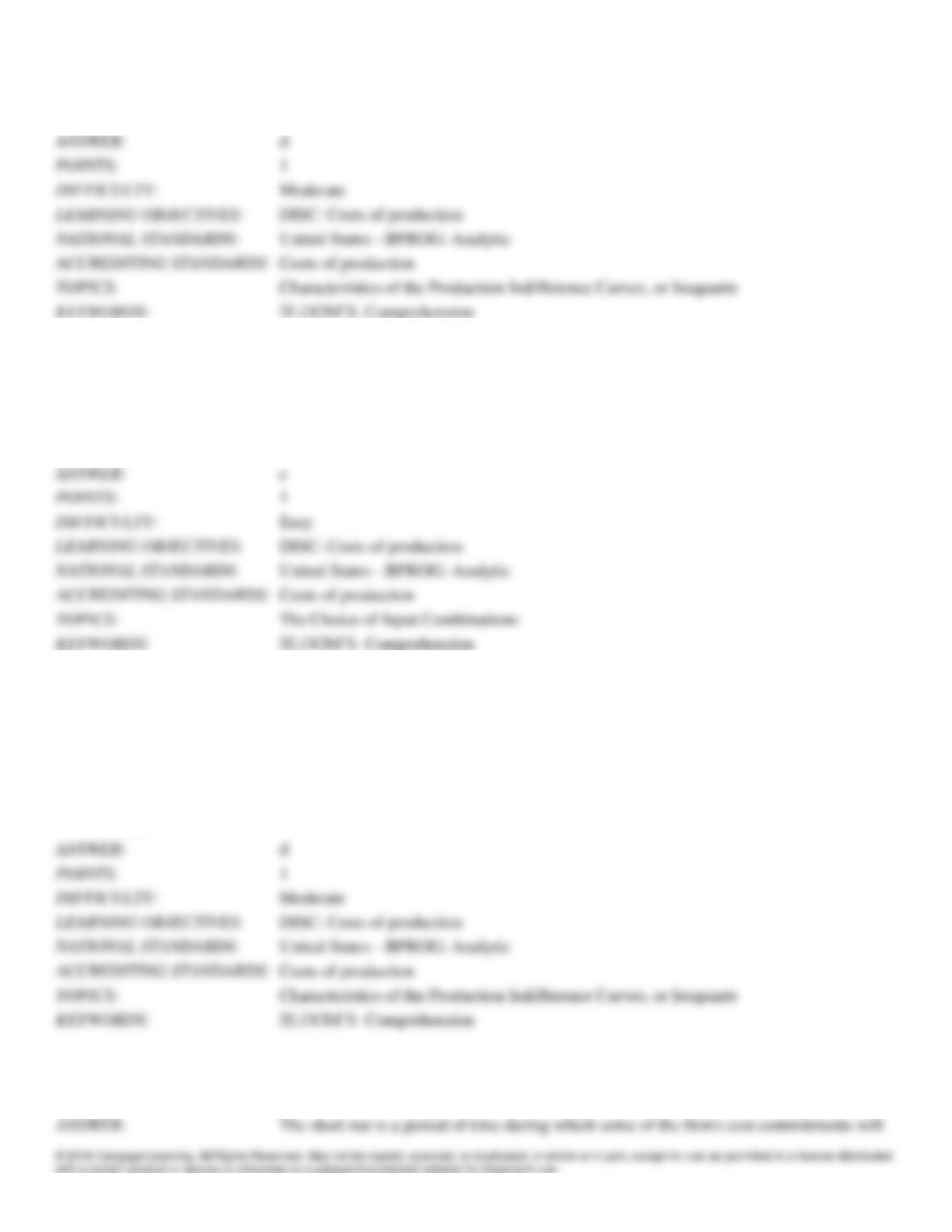
Figure 7-17
195. Which of the following statements must be true when a firm makes choices that put it at point A in Figure 7-17?
a.
The firm is minimizing its cost of producing 100 units of output.
b.
The ratio of the marginal physical products of labor and of land equals the ratio of the prices of labor and of
land.
c.
The firm first decided how much output to produce and then decided how to produce it.
d.
All of the above are true.
Moderate
DISC: Costs of production
United States – BPROG: Analytic
Costs of production
Characteristics of the Production Indifference Curves, or Isoquants
196. A firm that is seeking to minimize costs to produce a certain output:
a.
has a fixed budget
b.
has a large budget
c.
wants to use the smallest possible budget possible
d.
wants to use the same budget as that used last year
c
Easy
DISC: Costs of production
United States – BPROG: Analytic
Costs of production
The Choice of Input Combinations
197. With regard to the characteristics of production indifference curves, which of the following statements is/are NOT
true?
a.
Higher curves correspond to larger outputs.
b.
An indifference curve will generally have a negative slope.
c.
An indifference curve is typically assumed to curve inward toward the origin near its middle.
d.
All of the above are true for production indifference curves, but not for isoquants.
e.
b and c
Moderate
DISC: Costs of production
United States – BPROG: Analytic
Costs of production
Characteristics of the Production Indifference Curves, or Isoquants
Essay
198. Differentiate between the short run and the long run.
The short run is a period of time during which some of the firm’s cost commitments will
Easy
199. “If it were not for the law of diminishing marginal returns, the world’s wheat could be grown in a flower pot.”
Explain.
1
Moderate
200. The following table depicts the production relationship between units of labor and output of pepper on Pietrov’s
Pepper Farm.
Labor
Peppers
Labor
Peppers
1
10
6
75
2
25
7
77
3
45
8
78
4
60
9
77
5
70
10
75
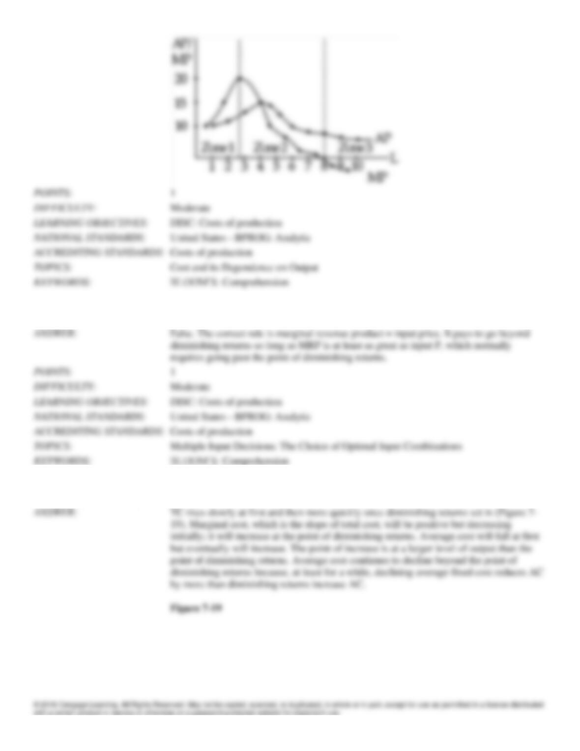
Graphically show the three zones of production corresponding to increasing, decreasing, and negative marginal product,
noting the point of diminishing returns.
201. “A producer wanting to employ optimal quantity of inputs should choose the point where diminishing returns sets
in.” True or false?
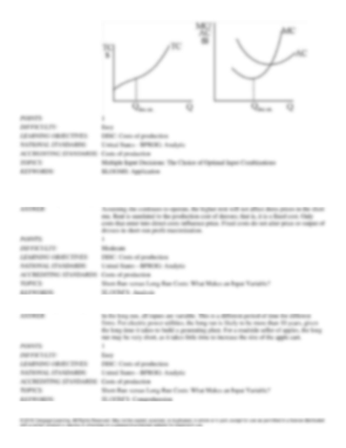
202. Graph typical total, average, and marginal cost curves and explain how their shapes are influenced by the law of
diminishing returns. Graph TC on a separate graph, AC and MC on a second graph.
203. Aunt Rose owned a dress shop on 81st Street and Broadway in Manhattan, selling limited-edition dresses to wealthy
clients. One day, her landlord tripled her rent. What effect would this have on her dress price in the short run, assuming
she is following the rules of profit maximization?
204. How long is the long run?
205. What is the shape of average cost curve? Provide the reason for that particular shape.
206. “Assuming the long-run average cost curve is U-shaped, a firm will always seek to operate at the lowest point on the
long-run average cost curve.” True or false?
207. Labor is available at a wage of $10. The last worker hired by Cal’s Corn Farm added 20 ears of corn, which Cal has
priced at four ears for $1. What advice would you give Cal?
208. Explain why the long-run average cost is typically U-shaped.
209. Peter Piper picks a peck of pickled peppers using 10 units of labor and two pepper-picking machines. The last worker
hired picked 100 peppers, and the last machine added 1,000 peppers. If labor can be hired at $5 a pepper picker and
machines cost $5,000, what advice do you have for Peter Piper?
210. If the MRP per dollar is greater for labor than that for tools, a producer should spend more money on labor than
originally planned and less on tools. How long can he continue this switch in spending? Why?
211. The United Auto Workers union is largely responsible for the historically high pay of American auto workers by
negotiating pay raises above those obtained by workers in other industries. In addition to increasing the pay of auto
workers, what other long-run effect would this high pay have on the use of auto workers?
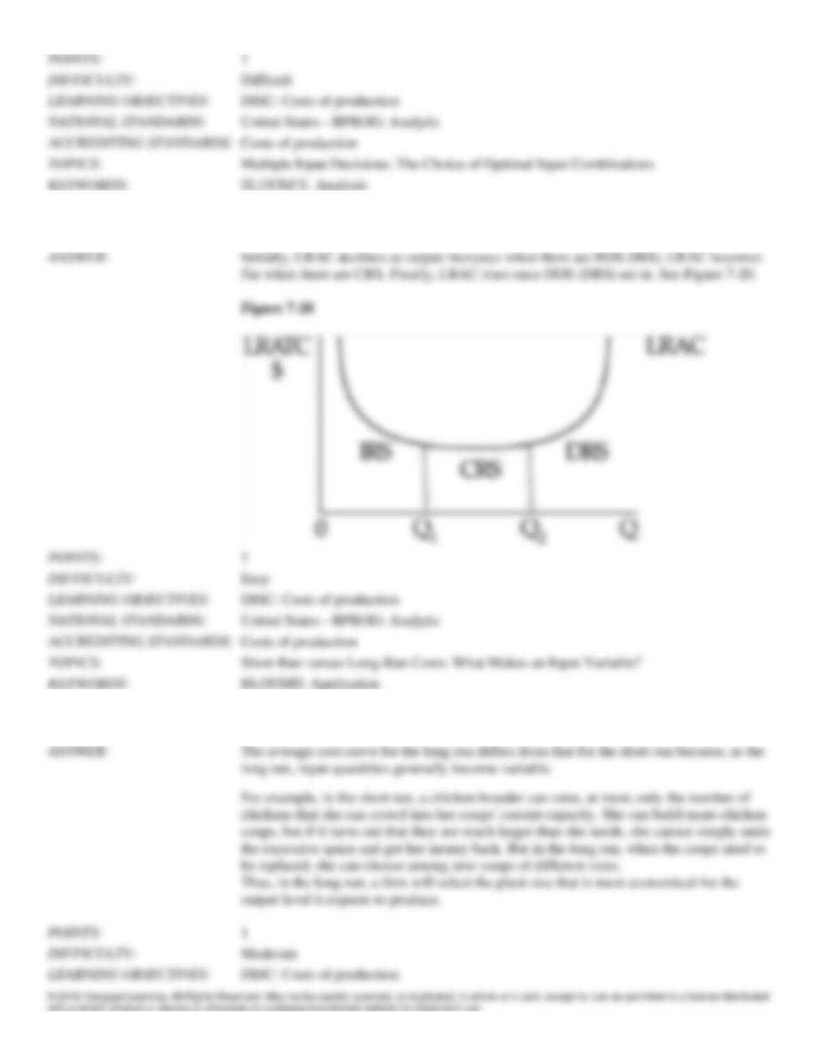
212. Draw a long-run average cost curve that first exhibits increasing returns to scale (economies of scale), then constant
returns to scale, and finally decreasing returns to scale (diseconomies of scale). Label each region.
213. Explain why the average cost curve for the long run differs from that for the short run.
United States – BPROG: Analytic
Costs of production
Cost and Its Dependence on Output
214. “Optimal input curve analysis is useless. Since firms never know the demand for their product with certainty, they
will rarely operate at the optimal input combination.” Agree or disagree?
1
Easy
DISC: Costs of production
United States – BPROG: Analytic
Costs of production
Multiple Input Decisions: The Choice of Optimal Input Combinations
215. Give a short concise definition for the following terms and explain their relationship to the study of economics.
a.
marginal physical product
b.
marginal revenue product
c.
law of diminishing returns
d
economies of scale
the price of the input.
1
Moderate
DISC: Costs of production
United States – BPROG: Reflective Thinking – BPROG: Analysis
Costs of production
Production, Input Choice, and Cost with One Variable Input
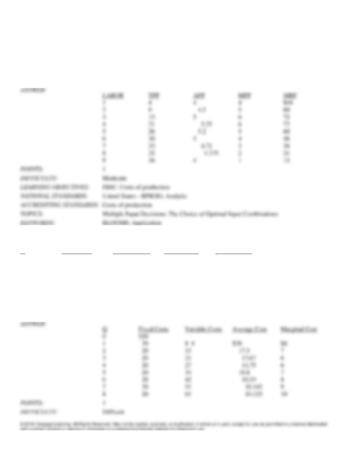
216. The table below gives data on output for a firm in the short run. The firm is able to hire labor and its TPP is given.
Compute the APP, MPP, and MRP for labor if the price of the good is fixed at $12 per unit.
LABOR
TPP
APP
MPP
MRP
1
4
_____
_____
_____
2
9
_____
_____
_____
3
15
_____
_____
_____
4
21
_____
_____
_____
5
26
_____
_____
_____
6
30
_____
_____
_____
7
33
_____
_____
_____
8
35
_____
_____
_____
9
36
_____
_____
_____
LABOR
APP
MRP
1
4
4
4
$48
2
9
4.5
5
60
3
15
5
6
72
4
21
5.25
6
72
5
26
5.2
5
60
6
30
5
4
48
7
33
4.71
3
36
8
35
4.375
2
24
9
36
4
1
12
1
Moderate
DISC: Costs of production
United States – BPROG: Analytic
Costs of production
Multiple Input Decisions: The Choice of Optimal Input Combinations
BLOOMS: Application
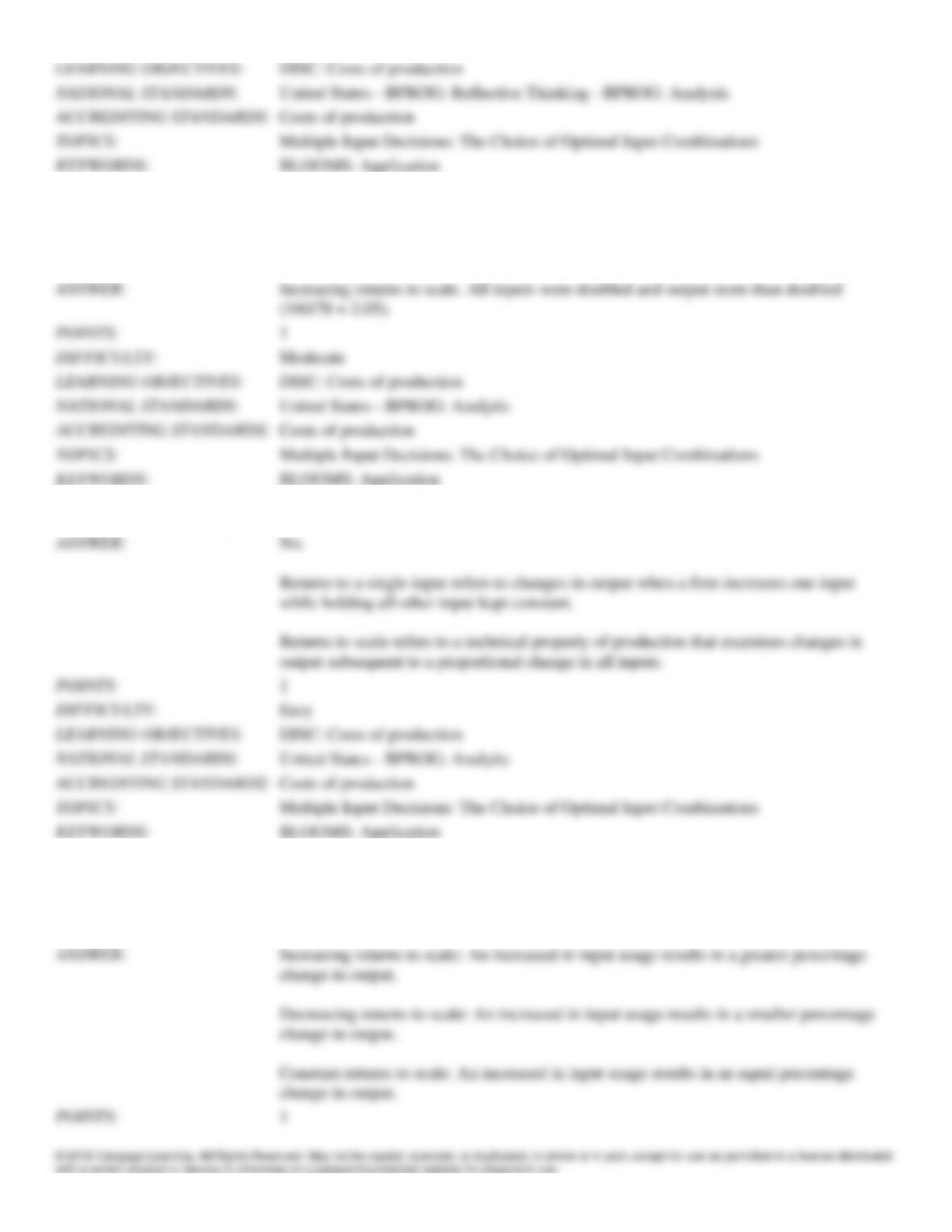
217. Complete the table below by computing the missing numbers from those that are given.
Q
Fixed Costs
Variable Costs
Average Cost
Marginal Cost
0
$20
_____
_____
_____
1
_____
_____
_____
$8
2
_____
$15
_____
_____
3
_____
_____
$13.67
_____
4
_____
_____
_____
6
5
_____
_____
_____
7
6
_____
42
_____
_____
7
_____
51
_____
_____
8
_____
_____
10.125
_____
Q
Fixed Costs
Variable Costs
Average Cost
Marginal Cost
0
$20
1
20
$ 8
$28
$8
2
20
15
17.5
7
3
20
21
13.67
6
4
20
27
11.75
6
5
20
34
10.8
7
6
20
42
10.33
8
7
20
51
10.143
9
8
20
61
10.125
10
1
Difficult
DISC: Costs of production
United States – BPROG: Reflective Thinking – BPROG: Analysis
Costs of production
Multiple Input Decisions: The Choice of Optimal Input Combinations
BLOOMS: Application
218. A.B. Denson Company had been employing 6 workers and 8 tons of raw materials, using 2,000 square feet of plant
space. The firm increased its work force to 12 workers utilizing 16 tons of raw materials in a plant space increased to
4,000 square feet. Total number of units of output increased from 78 to 160. What kind of returns to scale is the firm
experiencing? Defend your answer.
Moderate
DISC: Costs of production
United States – BPROG: Analytic
Costs of production
Multiple Input Decisions: The Choice of Optimal Input Combinations
BLOOMS: Application
219. Are returns to a single input and returns to scale one and the same? Explain.
Easy
DISC: Costs of production
United States – BPROG: Analytic
Costs of production
Multiple Input Decisions: The Choice of Optimal Input Combinations
BLOOMS: Application
220. Explain briefly the following concepts:
(a)
Increasing returns to scale.
(b)
Decreasing returns to scale.
(c)
Constant returns to scale.
221. Draw a graph using production indifference curves and budget lines showing a firm initially minimizing cost with its
inputs of A and B. Then illustrate a new optimal combination of inputs when the prices of the inputs change.