Chapter 06 – Consumer Behavior (+ Appendix)
6-55
135. In the diagram above, suppose the consumer is currently exhausting his or her income at
a point where the marginal rate of substitution of apples for oranges is greater than 5/4. That
is, MUA/MU0> 5/4. To maximize utility, the consumer should move from point:
Chapter 06 – Consumer Behavior (+ Appendix)
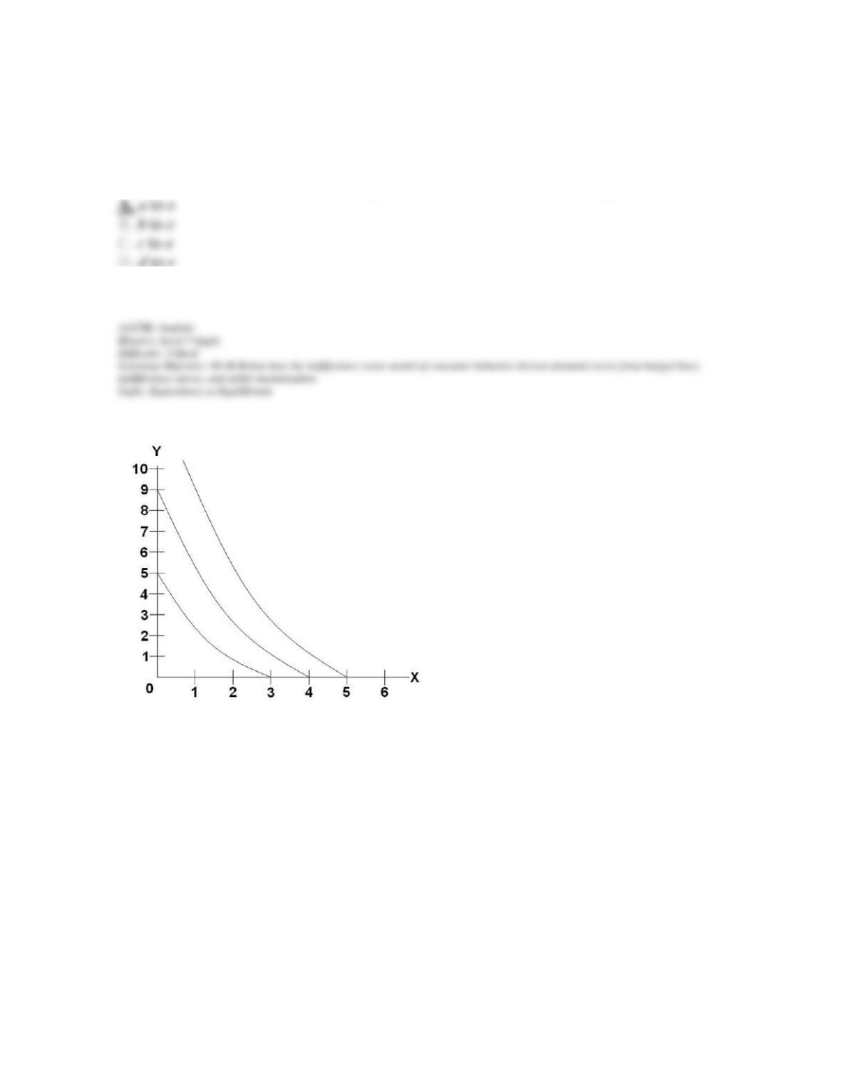
136. Refer to the above graph. Suppose you had tastes as described by the indifference curves
above. If your income was $100, Px = 20 and Py = 25, which combination of X and Y would
maximize your utility?
137. Refer to the above graph. Suppose you had tastes as described by the indifference curves
above. If your income was $90, Px = 30 and Py = 10, which combination of X and Y would
maximize your utility?
Chapter 06 – Consumer Behavior (+ Appendix)
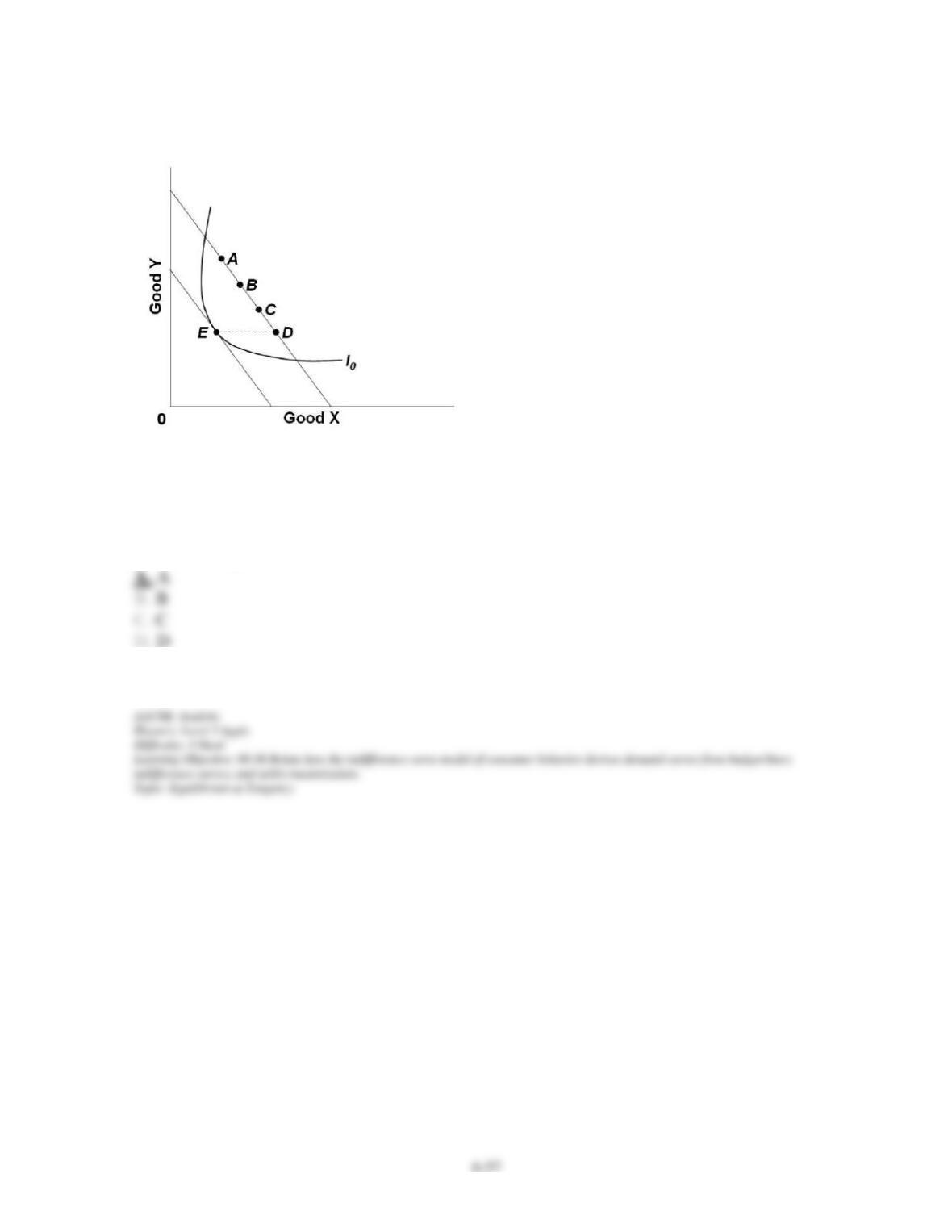
138. Consider the diagram above, where E is the consumer’s original equilibrium position. We
know good X is not a normal good if, as income increases, the consumer’s new equilibrium
position is at point:
Chapter 06 – Consumer Behavior (+ Appendix)
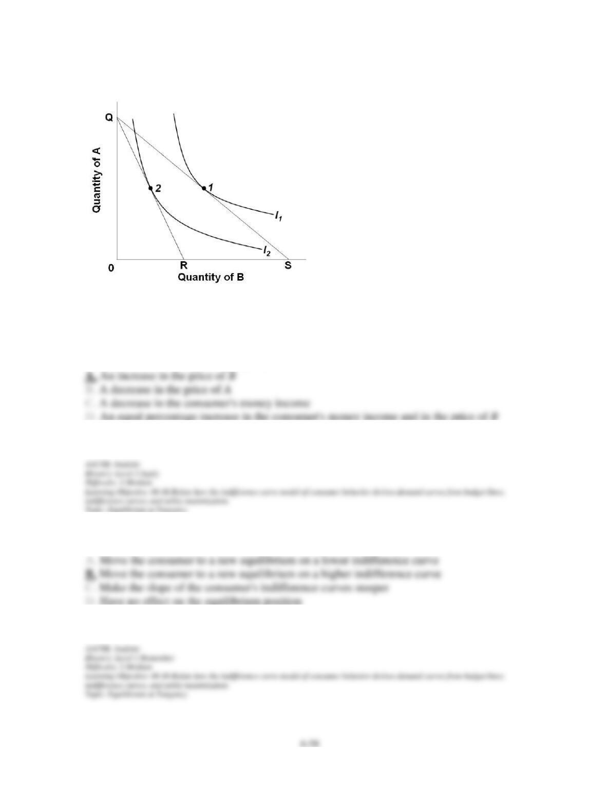
139. The graph above shows two indifference curves and QR and QS represent different
budget lines. A change in the equilibrium position on the diagram from point 1 to point 2
could result, other things being equal, from:
140. If a consumer is initially in equilibrium, an increase in money income will:
Chapter 06 – Consumer Behavior (+ Appendix)
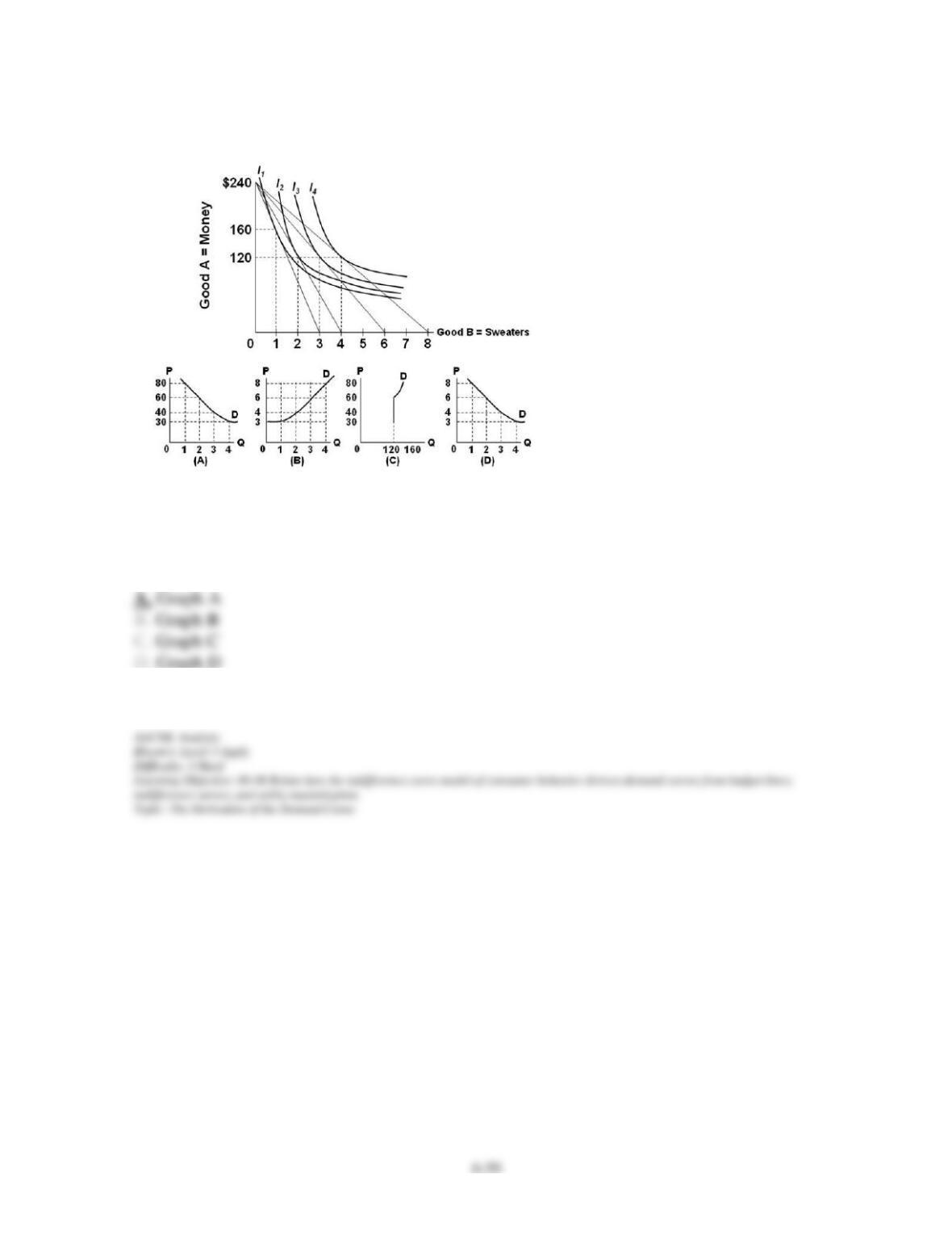
141. Given the indifference map and budget constraint lines above, what is the demand curve
for sweaters?
Chapter 06 – Consumer Behavior (+ Appendix)
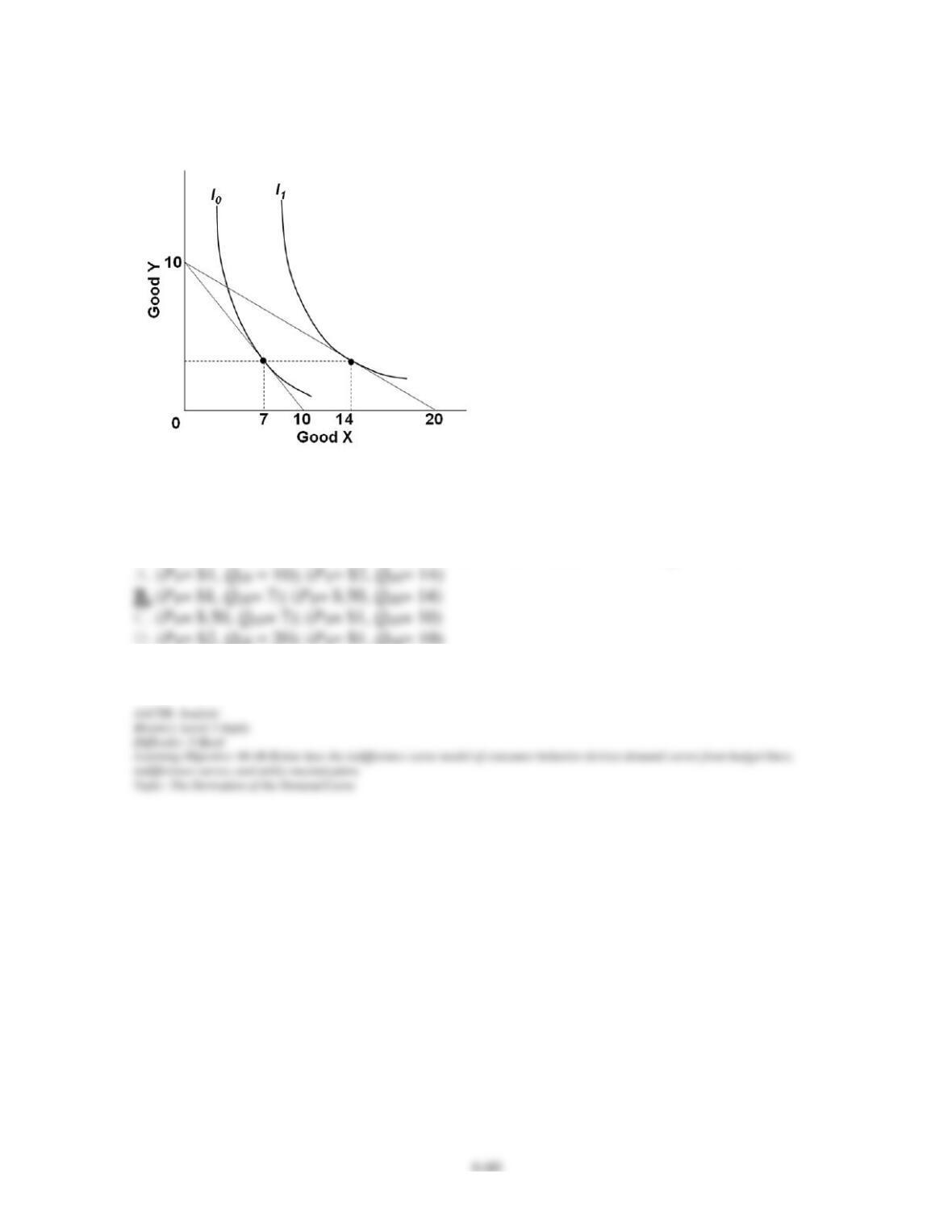
142. Given the indifference curves for an individual as shown above, if the price of good Y =
$1, it can be determined that two points on his or her demand curve for good X are:
Chapter 06 – Consumer Behavior (+ Appendix)
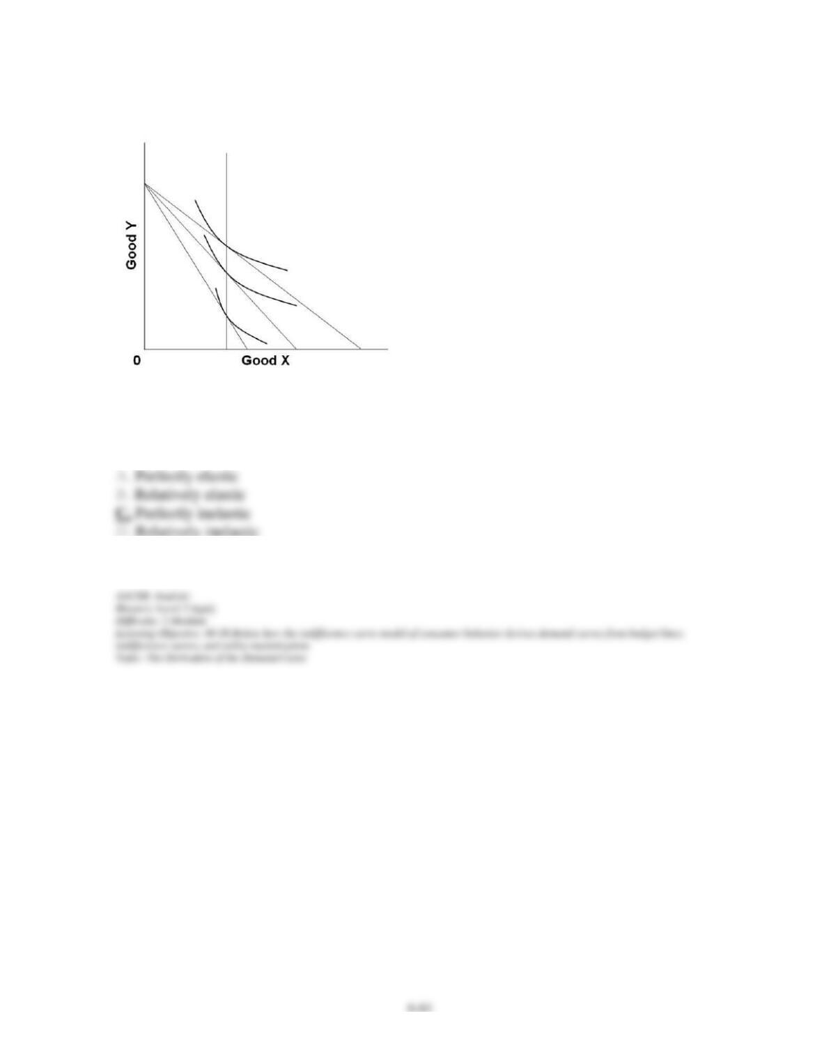
143. The individual demand curve that is implied by the budget constraints and indifference
curves above will be:
Chapter 06 – Consumer Behavior (+ Appendix)
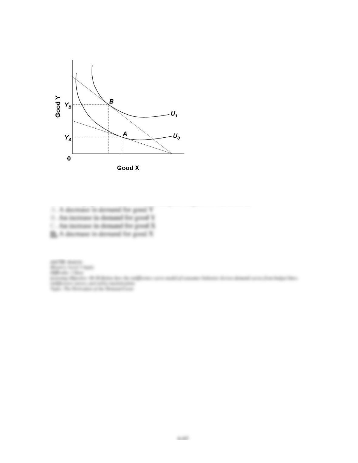
144. In the graph above, a decrease in the price of good Y will result in:
Chapter 06 – Consumer Behavior (+ Appendix)
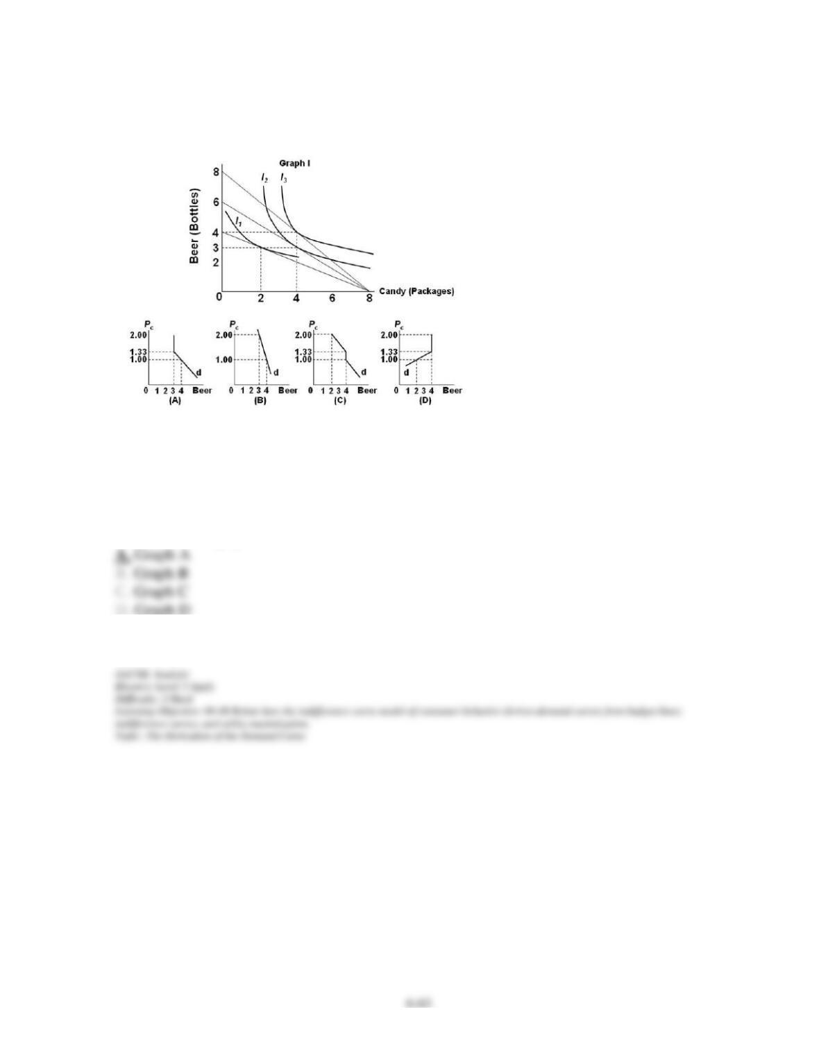
145. Graph I above shows E.T.’s equilibrium choices of beer and candy for three different
prices of beer. (I1, I2, and I3 are indifference curves. The price of a package of candy is
constant at $1.00.) Letting PC represent the price of beer, which demand curve (d) above is
consistent with graph I?
Chapter 06 – Consumer Behavior (+ Appendix)
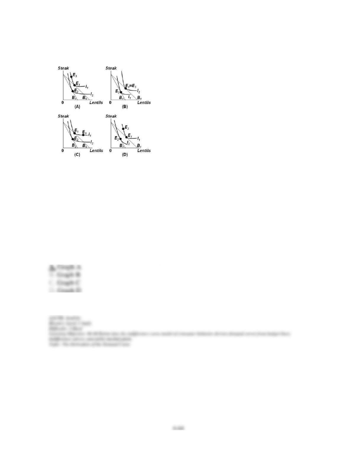
146. Recently the price of lentil beans increased. As a result Lincoln residents noticed that
their neighbor, Rasputin, increased his consumption of lentils and decreased his consumption
of steak. Rasputin said his utility had declined. Many citizens made donations to the
“Rasputin Relief Fund.” Rasputin was given a cash grant equal to the amount he claimed to
need to regain his initial utility level. Happy and thankful, Rasputin rushed off to the store to
make his new purchases. Each graph above shows two indifference curves for Rasputin, I1
and I2, and the two budget constraints, B1 and B2, that he faced. Let E1 represent Rasputin’s
initial equilibrium, E2 equal his equilibrium following the increase in the price of lentils, E3
his equilibrium after receiving the cash from the relief fund. Which graph above is consistent
with Rasputin’s claims in the above story?
Chapter 06 – Consumer Behavior (+ Appendix)
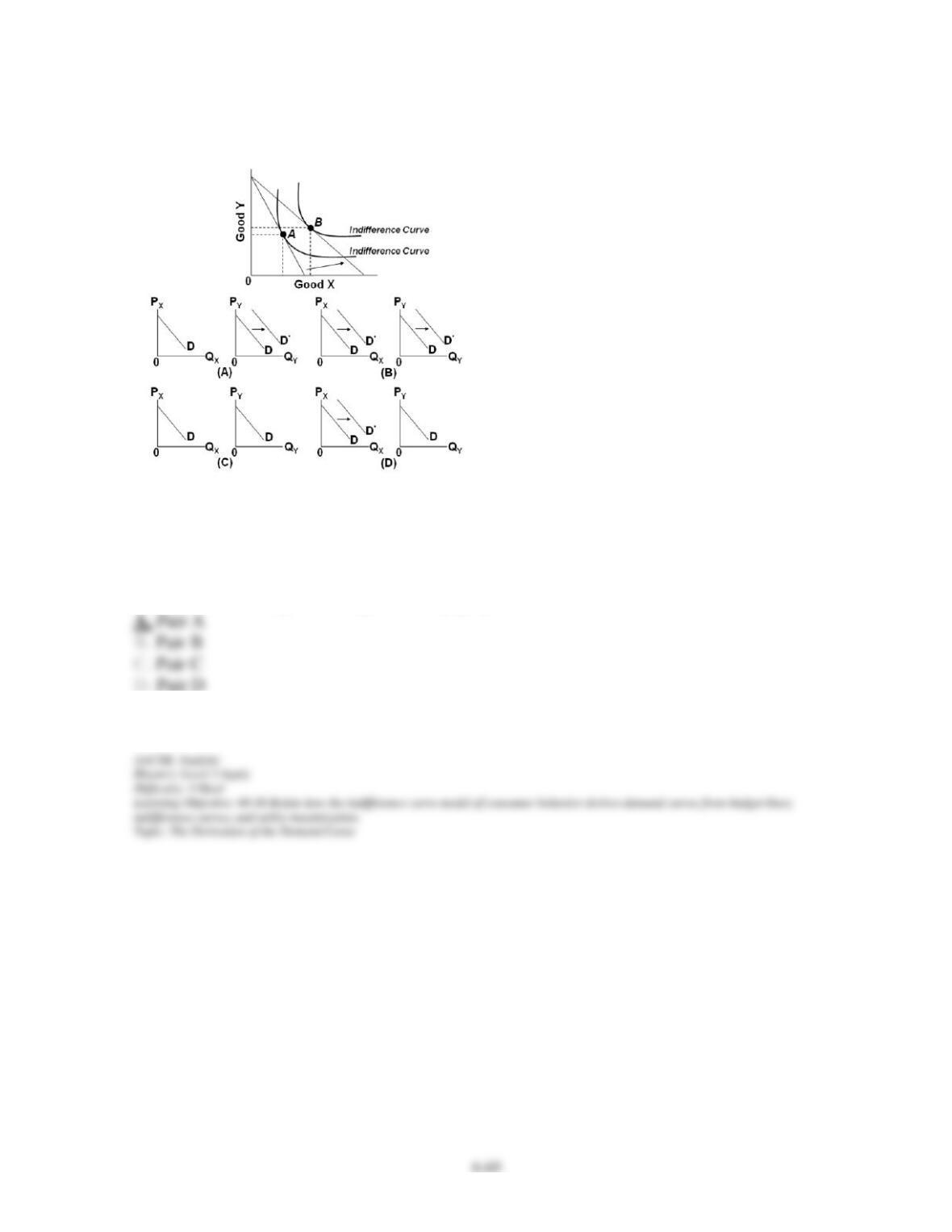
147. Suppose an individual’s budget line moved as shown above. Which of the four pairs of
graphs, each showing the demand for Good X and a separate demand for Good Y, is the most
consistent with the given change in the top graph?
Chapter 06 – Consumer Behavior (+ Appendix)
148. In a topographic map, each line represents a particular elevation above sea level, and in
an indifference map each line represents a particular level of:
149. The budget line shows all the combinations of two products which the consumer can
buy, given money income and product prices.
150. If the quantity of X is measured on the horizontal axis and the quantity of Y on the
vertical, then the slope of the budget line is equal to the price of X divided by the price of Y.
Chapter 06 – Consumer Behavior (+ Appendix)
151. A parallel shift in a budget line is caused by changes in a consumer’s level of
satisfaction.
152. A change in the relative prices for two goods can be shown as a parallel shift in a
consumer’s budget line.
153. Indifference curves are convex to the origin due to diminishing marginal rates of
substitution.
154. Indifference curves and budget lines can be used to derive an individual’s demand curve
for a product.
Chapter 06 – Consumer Behavior (+ Appendix)
155. The consumer will select that point on the budget line which puts the consumer on the
highest attainable indifference curve.
156. A consumer maximizes total utility when she or he purchases the combination of the two
products at which her or his budget line is tangent to an indifference curve.
157. An increase in the price of a product normally enables a consumer to reach a higher
indifference curve.
158. It is possible that as a result of the budget line shifting outwards, the consumer will buy
less of a product.