6.3 Mathematical and Graphical Problems
1) Your econometrics textbook stated that there will be omitted variable bias in the OLS estimator unless
the included regressor, X, is uncorrelated with the omitted variable or the omitted variable is not a
determinant of the dependent variable, Y. Give an intuitive explanation for these two conditions.

21
2) You have obtained data on test scores and student–teacher ratios in region A and region B of your state.
Region B, on average, has lower student–teacher ratios than region A. You decide to run the following
regression
0 1 1 1 2 3 3i i i i i
Y X X X u
= + + + +
where
1
X
is the class size in region A,
2
X
is the difference in class size between region A and B, and
3
X
is the class size in region B. Your regression package shows a message indicating that it cannot estimate
the above equation. What is the problem here and how can it be fixed?
3) In the case of perfect multicollinearity, OLS is unable to calculate the coefficients for the explanatory
variables, because it is impossible to change one variable while holding all other variables constant. To
see why this is the case, consider the coefficient for the first explanatory variable in the case of a multiple
regression model with two explanatory variables:
2
1 2 2 1 2
1 1 1 1
12
22
1 2 1 2
1 1 1
ˆ
n n n n
i i i i i i i
i i i i
n n n
i i i i
i i i
y x x y x x x
x x x x
= = = =
= = =
−
=
−
(small letters refer to deviations from means as in
ii
z Z Z=−
).
Divide each of the four terms by
22
22
11
nn
ii
ii
xx
==
to derive an expression in terms of regression coefficients
from the simple (one explanatory variable) regression model. In case of perfect multicollinearity, what
would be R2 from the regression of
1i
X
on
2i
X
? As a result, what would be the value of the denominator
in the above expression for
1
?
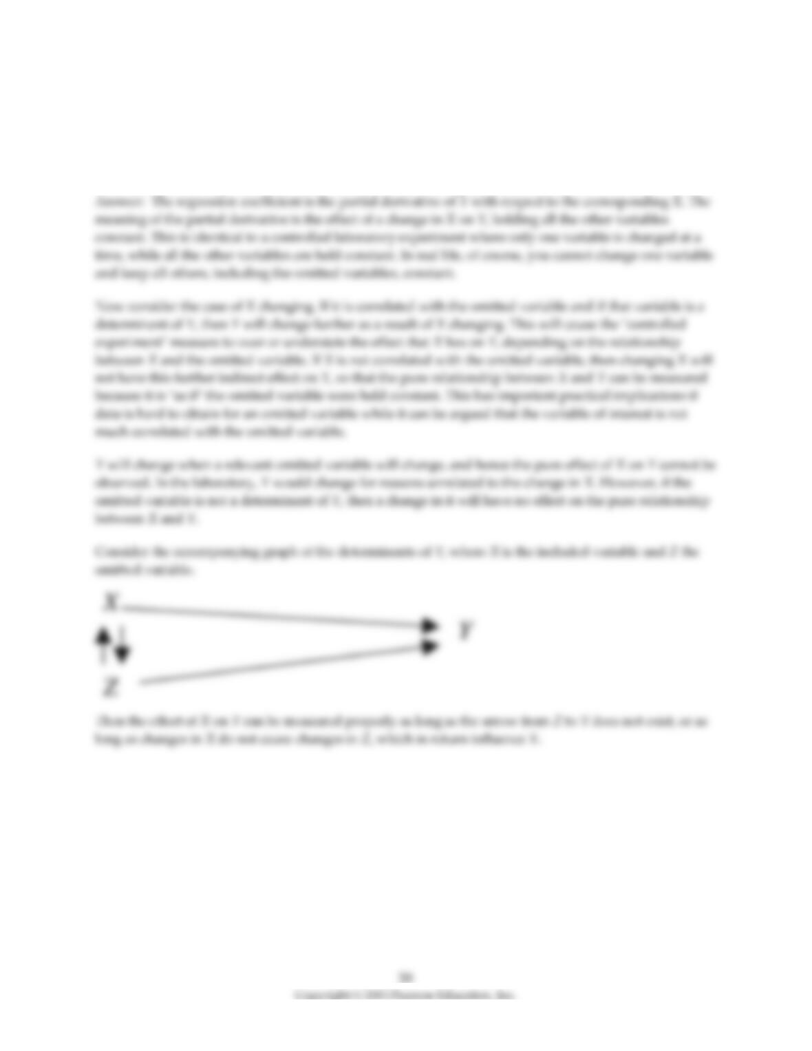
4) You try to establish that there is a positive relationship between the use of a fertilizer and the growth of
a certain plant. Set up the design of an experiment to establish the relationship, paying particular
attention to relevant control variables. Discuss in this context the effect of omitted variable bias.
5) In the multiple regression model with two regressors, the formula for the slope of the first explanatory
variable is
2
1 2 2 1 2
1 1 1 1
12
22
1 2 1 2
1 1 1
ˆ
n n n n
i i i i i i i
i i i i
n n n
i i i i
i i i
y x x y x x x
x x x x
= = = =
= = =
−
=
−
(small letters refer to deviations from means as in
ii
z Z Z=−
).
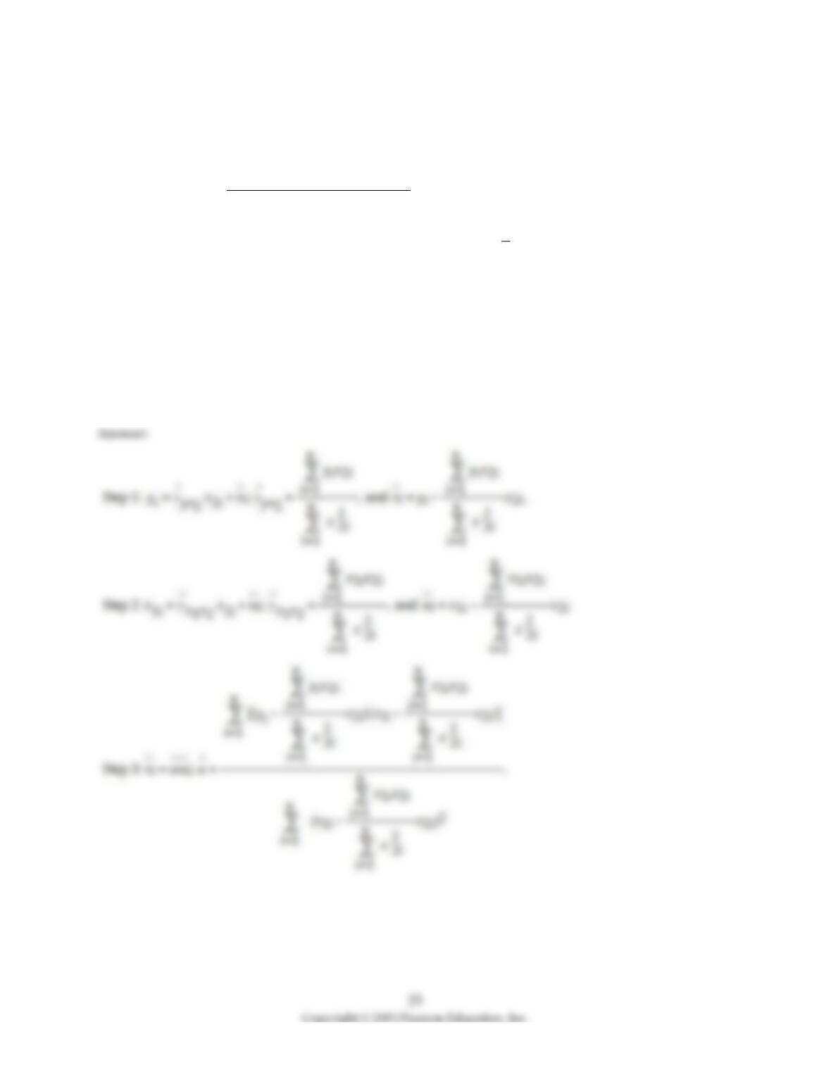
An alternative way to derive the OLS estimator is given through the following three step procedure.
Step 1: regress Y on a constant and
2
X
, and calculate the residual (Res1).
Step 2: regress
1
X
on a constant and
2
X
, and calculate the residual (Res2).
Step 3: regress Res1 on a constant and Res2.
Prove that the slope of the regression in Step 3 is identical to the above formula.
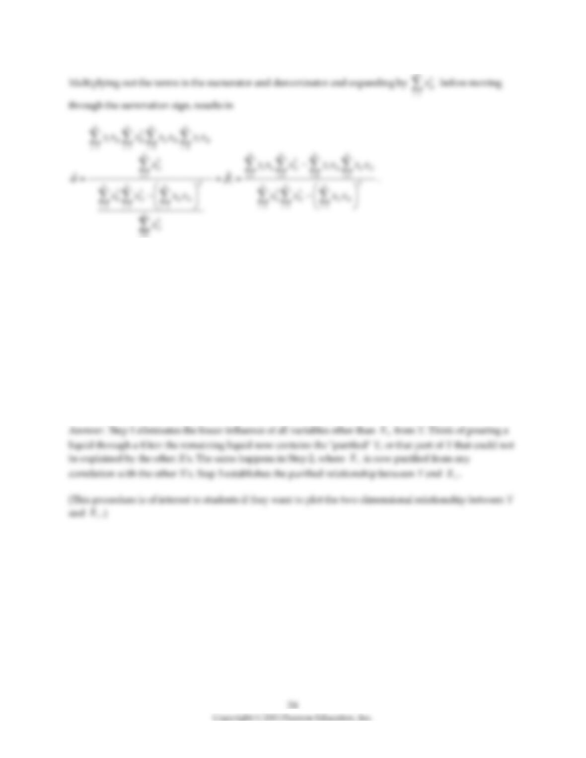
6) In the multiple regression problem with k explanatory variable, it would be quite tedious to derive the
formulas for the slope coefficients without knowledge of linear algebra. The formulas certainly do not
resemble the formula for the slope coefficient in the simple linear regression model with a single
explanatory variable. However, it can be shown that the following three step procedure results in the
same formula for slope coefficient of the first explanatory variable,
1
X
:
Step 1: regress Y on a constant and all other explanatory variables other than
1
X
, and calculate the
residual (Res1).
Step 2: regress
1
X
on a constant and all other explanatory variables, and calculate the residual (Res2).
Step 3: regress Res1 on a constant and Res2.
Can you give an intuitive explanation to this procedure?
1
X
1
X
1
X
1
X
7) Give at least three examples from macroeconomics and three from microeconomics that involve
specified equations in a multiple regression analysis framework. Indicate in each case what the expected
signs of the coefficients would be and if theory gives you an indication about the likely size of the
coefficients.
8) One of your peers wants to analyze whether or not participating in varsity sports lowers or increases
the GPA of students. She decides to collect data from 110 male and female students on their GPA and the
number of hours they spend participating in varsity sports. The coefficient in the simple regression
function turns out to be significantly negative, using the t–statistic and carrying out the appropriate
hypothesis test. Upon reflection, she is concerned that she did not ask the students in her sample whether
or not they were female or male. You point out to her that you are more concerned about the effect of
omitted variables in her regression, such as the incoming SAT score of the students, and whether or not
they are in a major from a high/low grading department. Elaborate on your argument.
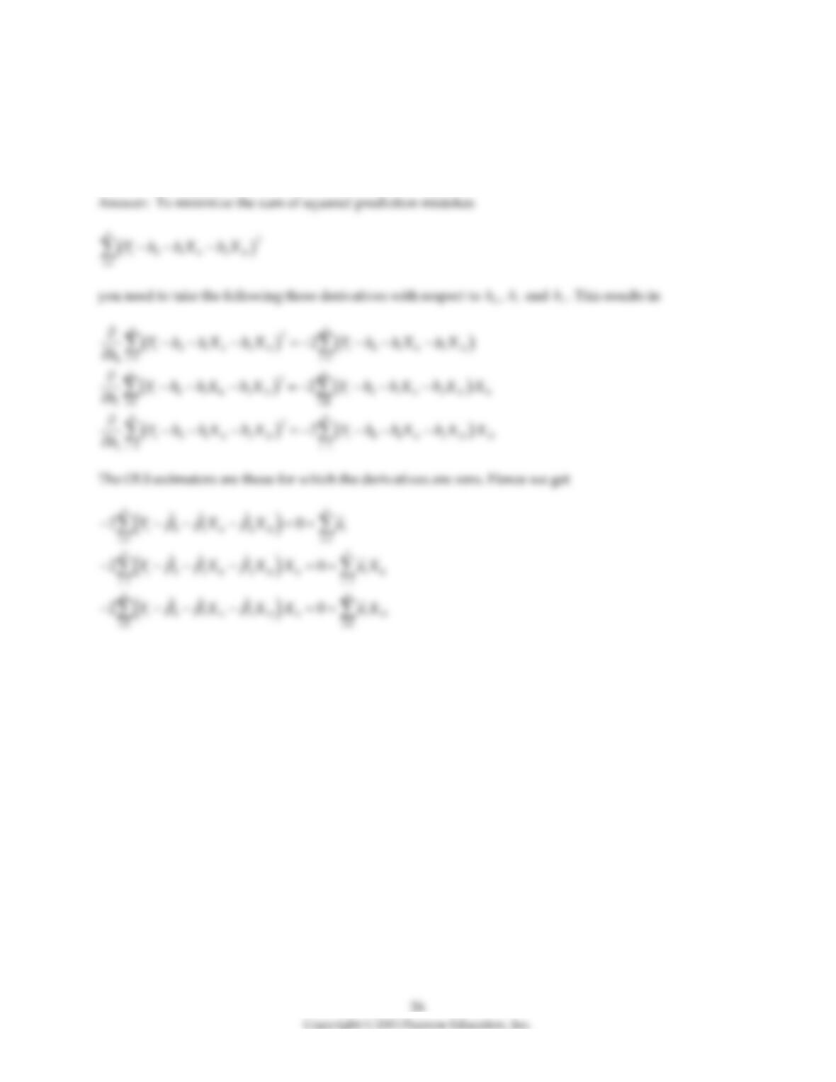
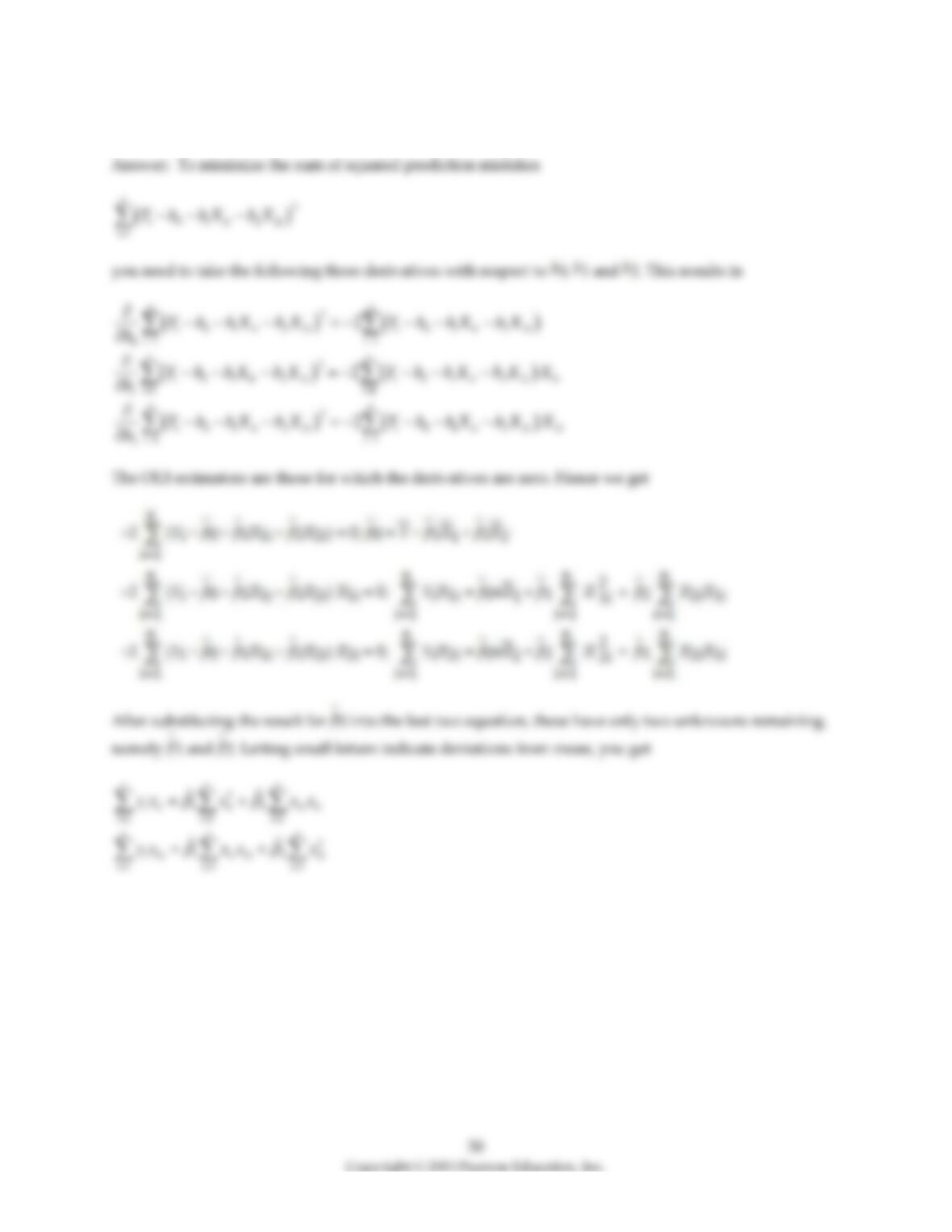
9) (Requires Calculus) For the case of the multiple regression problem with two explanatory variables,
show that minimizing the sum of squared residuals results in three conditions:
12
1 1 1
ˆ ˆ ˆ
0; 0; 0
n n n
i i i i i
i i i
u u X u X
= = =
= = =
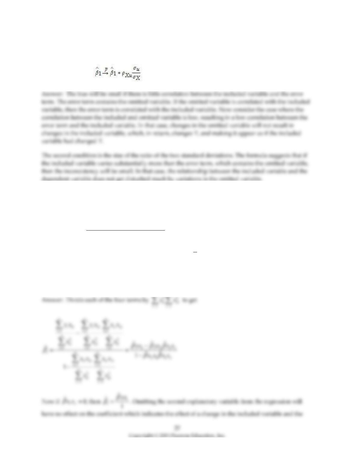
10) The probability limit of the OLS estimator in the case of omitted variables is given in your text by the
following formula:
Give an intuitive explanation for two conditions under which the bias will be small.
11) It is not hard, but tedious, to derive the OLS formulae for the slope coefficient in the multiple
regression case with two explanatory variables. The formula for the first regression slope is
2
1 2 2 1 2
1 1 1 1
12
22
1 2 1 2
1 1 1
ˆ
n n n n
i i i i i i i
i i i i
n n n
i i i i
i i i
y x x y x x x
x x x x
= = = =
= = =
−
=
−
(small letters refer to deviations from means as in
ii
z Z Z=−
).
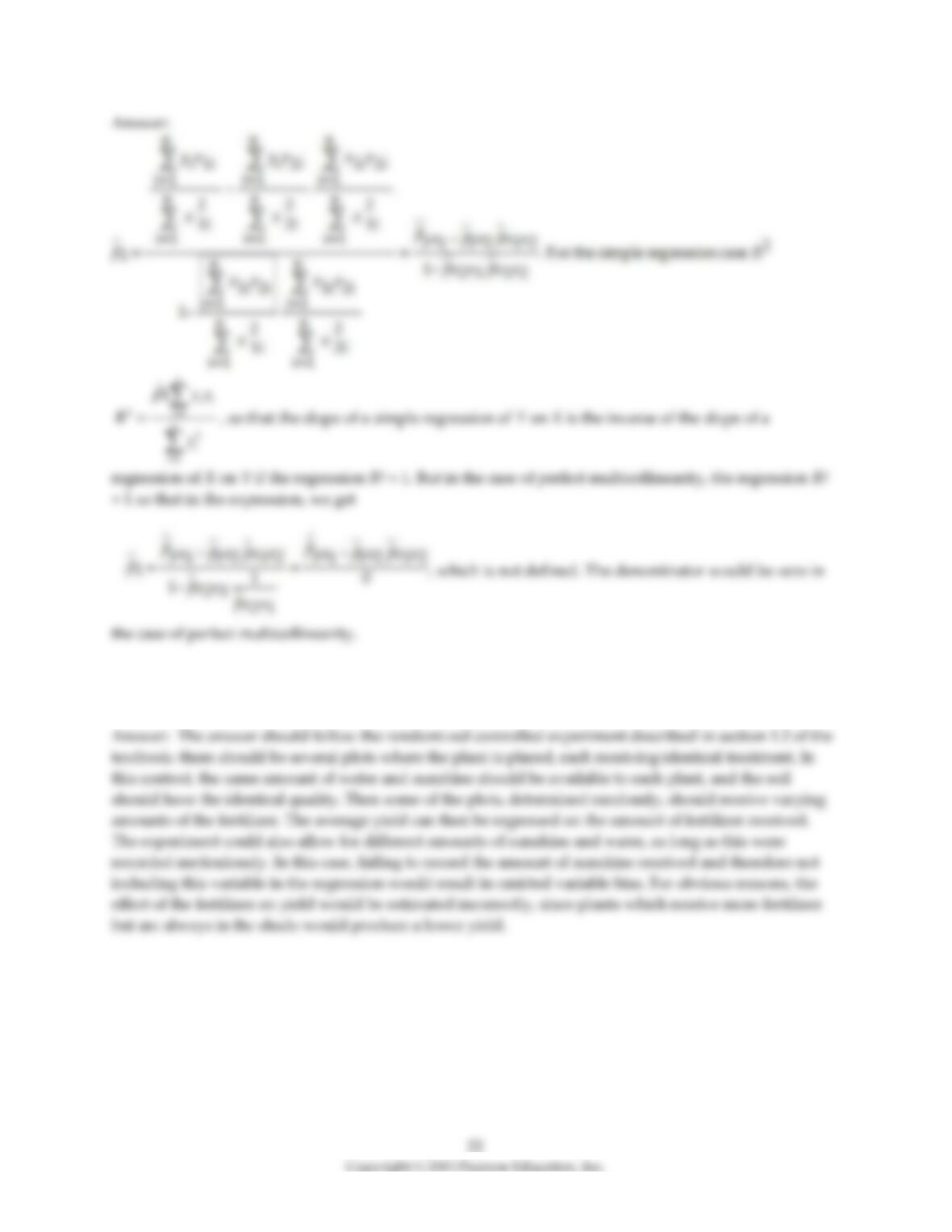
Show that this formula reduces to the slope coefficient for the linear regression model with one regressor
if the sample correlation between the two explanatory variables is zero. Given this result, what can you
say about the effect of omitting the second explanatory variable from the regression?
nn
12) (Requires Statistics background beyond Chapters 2 and 3) One way to establish whether or not there
is independence between two or more variables is to perform a
2
X
– test on independence between two
variables. Explain why multiple regression analysis is a preferable tool to seek a relationship between
variables.
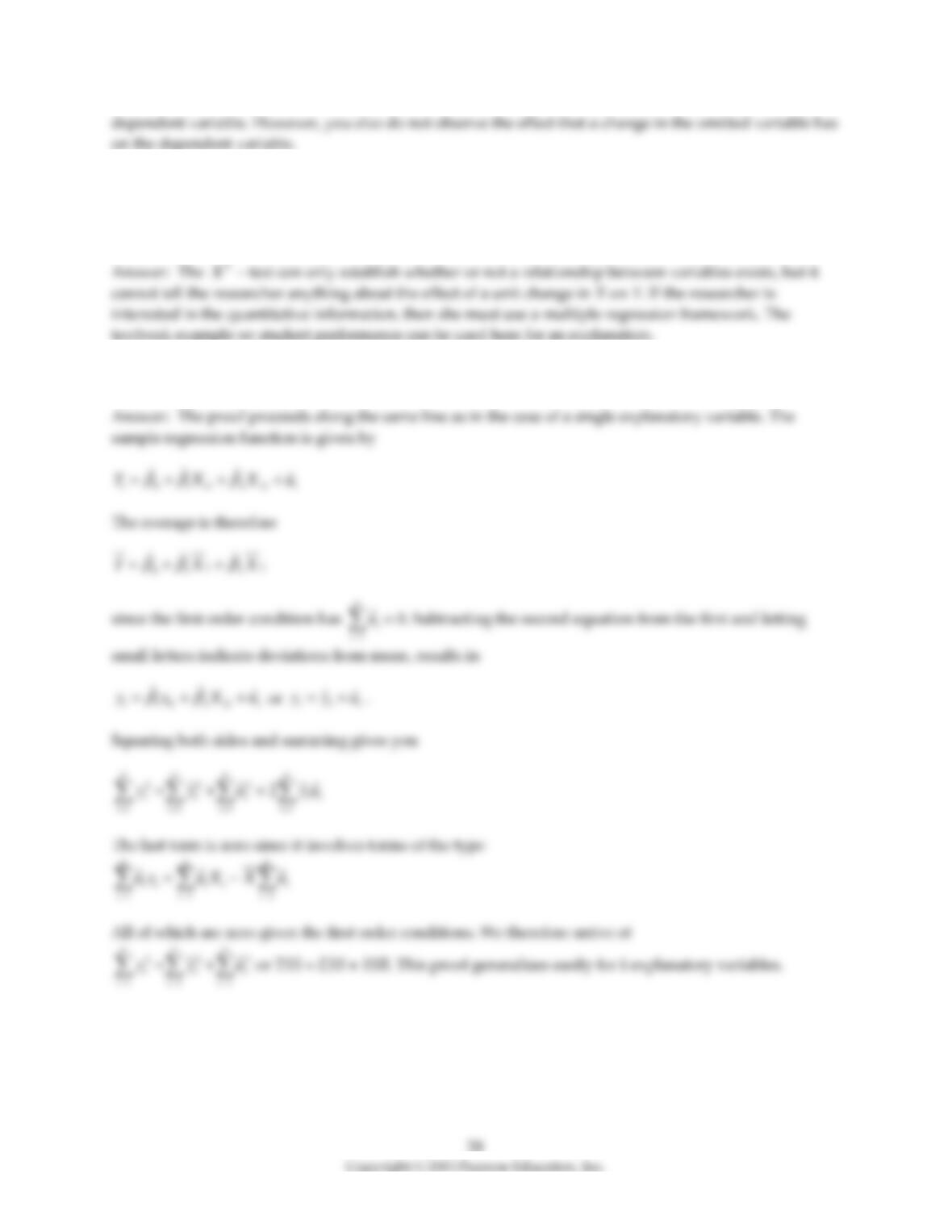
13) In the multiple regression with two explanatory variables, show that the TSS can still be decomposed
into the ESS and the RSS.

14) The OLS formula for the slope coefficients in the multiple regression model become increasingly more
complicated, using the “sums” expressions, as you add more regressors. For example, in the regression
with a single explanatory variable, the formula is
( )( )
( )
1
2
1
n
ii
i
n
i
i
X X Y X
XX
=
=
−−
−
whereas this formula for the slope of the first explanatory variable is
2
1 2 2 1 2
1 1 1 1
12
22
1 2 1 2
1 1 1
ˆ
n n n n
i i i i i i i
i i i i
n n n
i i i i
i i i
y x x y x x x
x x x x
= = = =
= = =
−
=
−
(small letters refer to deviations from means as in
ii
z Z Z=−
)
in the case of two explanatory variables. Give an intuitive explanations as to why this is the case.
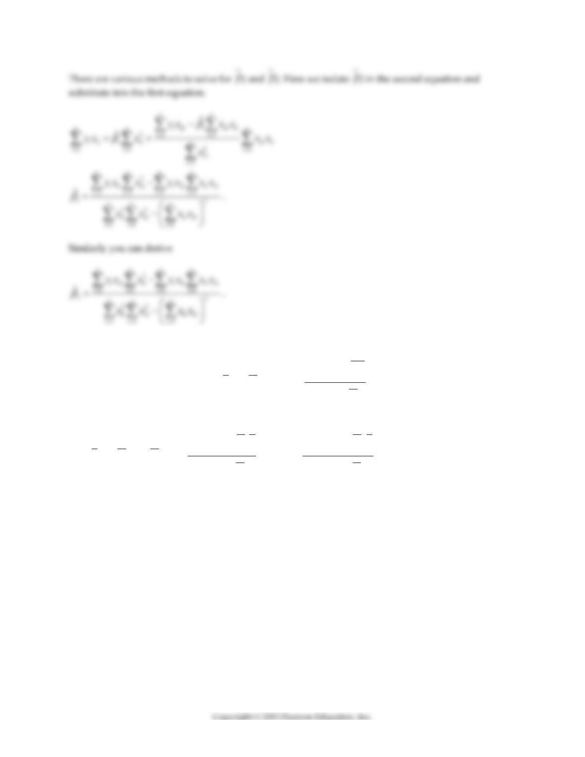
15) (Requires Calculus) For the case of the multiple regression problem with two explanatory variables,
derive the OLS estimator for the intercept and the two slopes.
31
16) (Requires Calculus) For the simple linear regression model of Chapter 4,
01i i i
Y X u
= + +
, the OLS
estimator for the intercept was
01
ˆˆ
YX
=−
, and
1
12
2
1
ˆ
n
ii
i
n
i
i
X Y nXY
X nX
=
=
−
=
−
. Intuitively, the OLS estimators
for the regression model
0 1 1 2 2i i i i
Y X X u
= + + +
might be
1
1
1
12
0 1 2 1 2
2
1
1
1
ˆ ˆ ˆ ˆ
,
n
ii
i
n
i
i
X Y n X Y
Y X X
X nX
=
=
−
= − − =
−
and
2
2
1
22
2
2
2
1
ˆ
n
ii
i
n
i
i
X Y n X Y
X nX
=
=
−
=
−
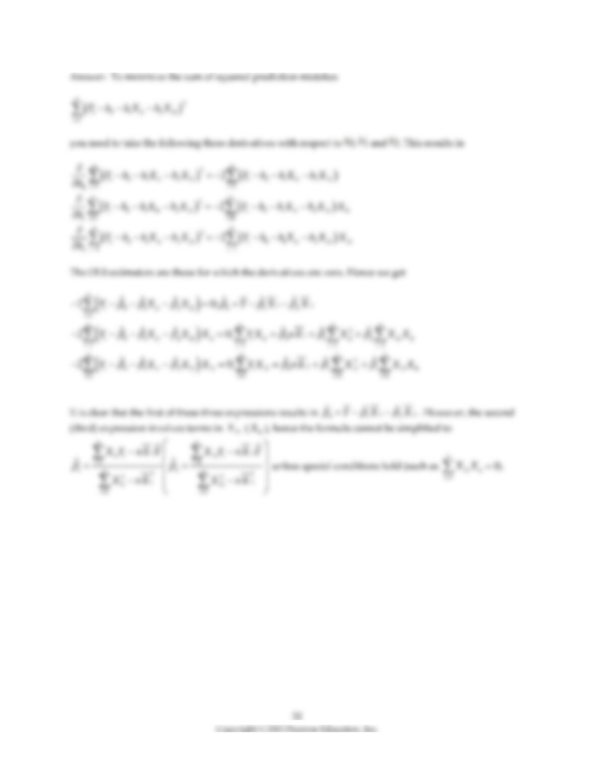
. By minimizing the prediction
mistakes of the regression model with two explanatory variables, show that this cannot be the case.
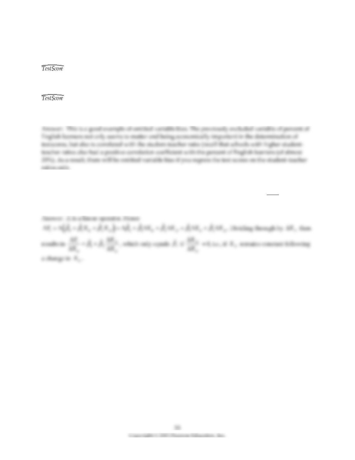
17) Your textbook extends the simple regression analysis of Chapters 4 and 5 by adding an additional
explanatory variable, the percent of English learners in school districts (PctEl). The results are as follows:
= 698.9 – 2.28 × STR
and
= 698.0 – 1.10 × STR – 0.65 × PctEL
Explain why you think the coefficient on the student–teacher ratio has changed so dramatically (been
more than halved).
18) (Requires some Calculus) Consider the sample regression function .
0 1 1 2 2
ˆ ˆ ˆ
i i i
Y X X
= + +
. Take the total derivative. Next show that the partial derivative
1
i
i
Y
X
is obtained
by holding
2i
X
constant, or controlling for
2i
X
.
2i
X
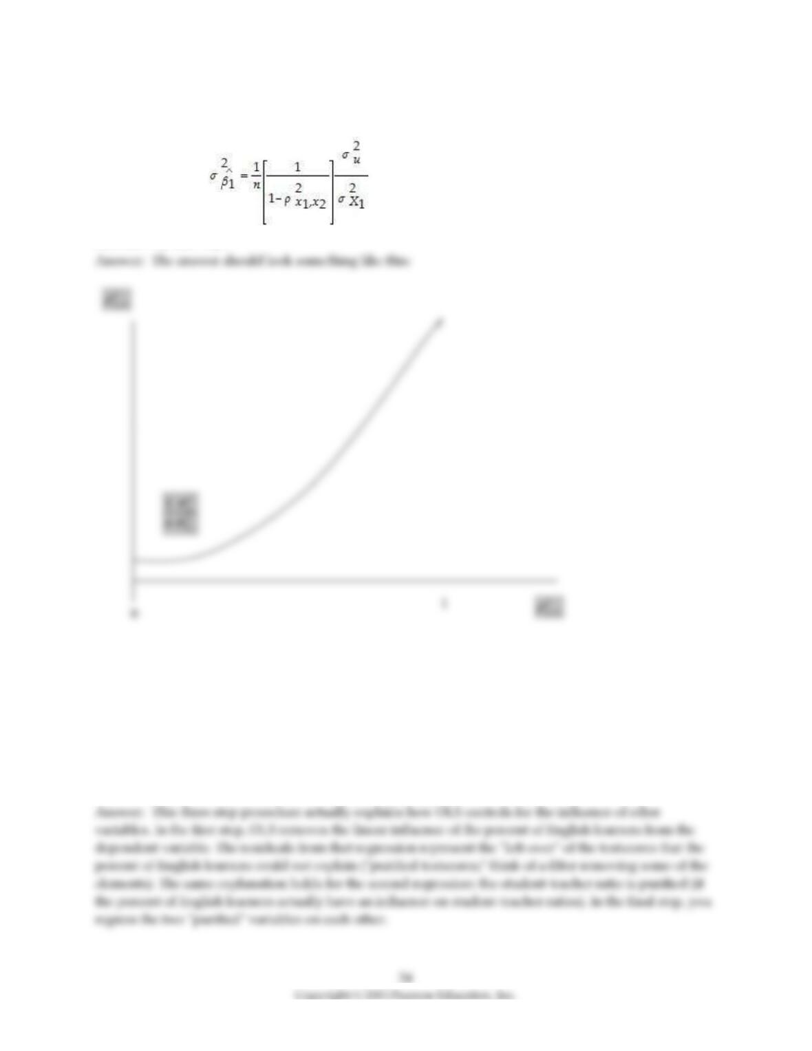
19) (Requires Appendix material) Consider the following population regression function model with two
explanatory variables:
0 1 1 2 2
ˆ ˆ ˆ
i i i
Y X X
= + +
. It is easy but tedious to show that SE(
2
ˆ
) is given by the
following formula: . Sketch how SE(
2
ˆ
) increases with the correlation
between
1i
X
and
2i
X
.
20) For this question, use the California Testscore Data Set and your regression package (a spreadsheet
program if necessary). First perform a multiple regression of testscores on a constant, the student–teacher
ratio, and the percent of English learners. Record the coefficients. Next, do the following three step
procedure instead: first, regress the testscore on a constant and the percent of English learners. Calculate
the residuals and store them under the name resYX2. Second, regress the student–teacher ratio on a
constant and the percent of English learners. Calculate the residuals from this regression and store these
under the name resX1X2. Finally regress resYX2 on resX1X2 (and a constant, if you wish). Explain
intuitively why the simple regression coefficient in the last regression is identical to the regression
coefficient on the student–teacher ratio in the multiple regression.
21) Assume that you have collected cross–sectional data for average hourly earnings (ahe), the number of
years of education (educ) and gender of the individuals (you have coded individuals as “1” if they are
female and “0” if they are male; the name of the resulting variable is DFemme).
Having faced recent tuition hikes at your university, you are interested in the return to education, that is,
how much more will you earn extra for an additional year of being at your institution. To investigate this
question, you run the following regression:
= –4.58 + 1.71×educ
N = 14,925, R2 = 0.18, SER = 9.30
a. Interpret the regression output.
b. Being a female, you wonder how these results are affected if you entered a binary variable (DFemme),
which takes on the value of “1” if the individual is a female, and is “0” for males. The result is as follows:
= –3.44 – 4.09×DFemme + 1.76×educ
N = 14,925, R2 = 0.22, SER = 9.08
Does it make sense that the standard error of the regression decreased while the regression R2 increased?
c. Do you think that the regression you estimated first suffered from omitted variable bias?
22) You have collected data on individuals and their attributes. Consequently you have generated several
binary variables, which take on a value of “1” if the individual has that characteristic and are “0”
otherwise. One example is the binary variable DMarr which is “1” for married individuals and “0” for non–
married variables. If you run the following regression:
ahei= β0 + β1×educi + β2×DMarri + ui
a. What is the interpretation for β2?
b. You are interested in directly observing the effect that being non–married (“single”) has on earnings,
controlling for years of education. Instead of recording all observations such that they are “1” for a not
married individual and “0” for a married person, how can you generate such a variable (DSingle) through
a simple command in your regression program?
23) Consider the following earnings function:
ahei= β0 + β1×DFemmei + β2×educi+…+ ui
versus the alternative specification
ahei= γ0 × DMale + γ1×DFemmei + γ2×educi+…+ ui
where ahe is average hourly earnings, DFemme is a binary variable which takes on the value of “1” if the
individual is a female and is “0″ otherwise, educ measures the years of education, and DMale is a binary
variable which takes on the value of “1” if the individual is a male and is “0” otherwise. There may be
additional explanatory variables in the equation.
a. How do the βs and γs compare? Putting it differently, having estimated the coefficients in the first
equation, can you derive the coefficients in the second equation without re–estimating the regression?
b. Will the goodness of fit measures, such as the regression R2, differ between the two equations?
c. What is the reason why economists typically prefer the second specification over the first?
24) You would like to find the effect of gender and marital status on earnings. As a result, you consider
running the following regression:
ahei= β0 + β1×DFemmei + β2×DMarri + β3×DSinglei + β4×educi+…+ ui
Where ahe is average hourly earnings, DFemme is a binary variable which takes on the value of “1” if the
individual is a female and is “0″ otherwise, DMarr is a binary variable which takes on the value of “1” if
the individual is married and is “0” otherwise, DSingle takes on the value of “1” if the individual is not
married and is “0” otherwise. The regression program which you are using either returns a message that
the equation cannot be estimated or drops one of the coefficients. Why do you think that is?