CHAPTER 6—FORECASTING Key
1. A 5% growth trend with annual compounding:
2. A forecast method based on the informed opinion of several individuals is called:
3. A rhythmic annual pattern in sales or profits is called:
4. Growth trend analysis assumes:
5. Lagging economic indicators include:
6. The Delphi method:
7. A secular trend is the:
8. Linear trend analysis assumes:
9. The forecasting technique least-suited for short term projection is:
10. Which of the following forecasting methods is not qualitative?
11. Time-series methods:
12. If an economic time series is growing by a constant dollar amount each period, the most accurate forecast
model is:
13. Social habits that produce an annual pattern in a time series result in:
14. Which of the following is a leading economic indicator?
15. Econometric methods:
16. A diffusion index that registers 40% indicates that:
17. Econometric forecasting methods:
18. The accuracy of an econometric forecast would be most questionable when the:
19. A panel consensus formed by providing feedback without direct identification of individual positions is
called:
20. Unpredictable shocks to the economic system are called:
21. A leading economic indicator of business cycle peaks is given by:
22. Qualitative methods and market experiments work best for forecasting product:
24. To predict the effects on a particular industry of changes in other sectors of the economy forecasters should
employ:
25. Which of the following does not indicate the relative accuracy of an economic forecast?
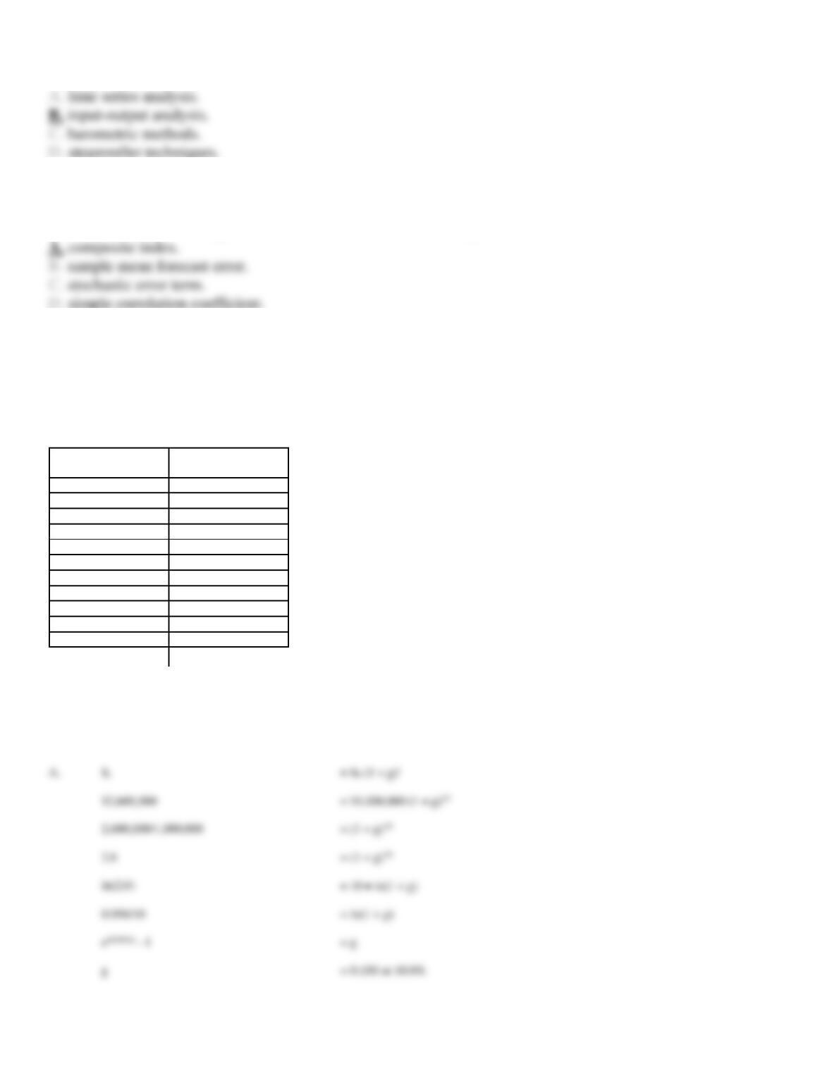
26. Annual Compounding. The following table shows annual sales data for Nanotechnology, Inc., over the
ten-year 1995-2005 period:
Year
Sales
($ Millions)
1995
$1.0
1996
1.1
1997
1.2
1998
1.2
1999
1.3
2000
1.4
2001
1.5
2002
1.9
2003
2.0
2004
2.5
2005
2.6
A.
Calculate the 1995-2005 growth rate in sales using the constant rate of change model with annual compounding.
B.
Forecast sales for the years 2010 and 2015.
A.
$2,600,000
2,600,000/1,000,000
2.6
= 10 • ln(1 + g)
0.956/10
= ln(1 + g)
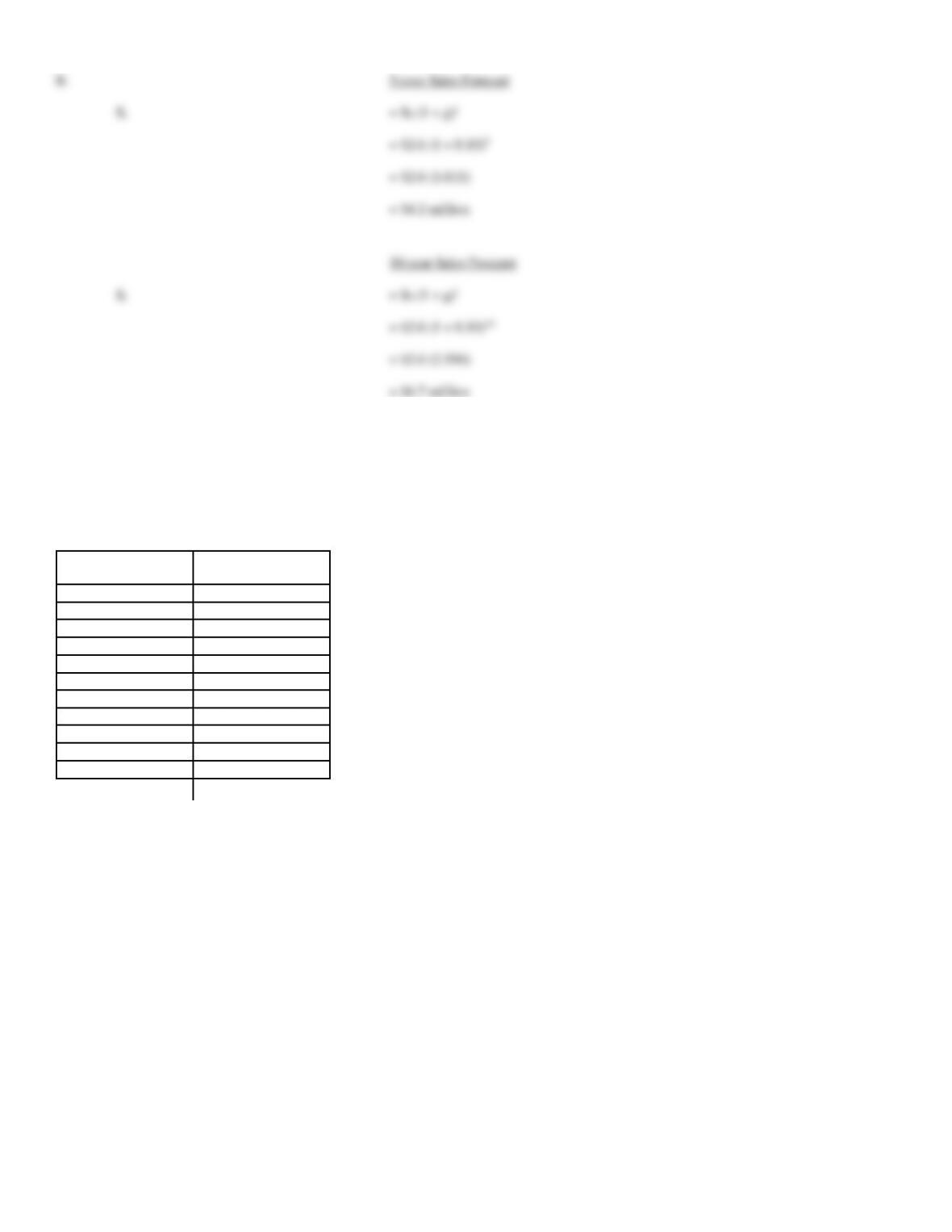
27. Annual Compounding. The following table shows annual sales data for Landrover, Inc., over the ten-year
1998-2008 period:
Year
Sales
($ Millions)
1998
$ 4.0
1999
4.8
2000
5.6
2001
6.4
2002
7.0
2003
7.6
2004
8.4
2005
9.2
2006
10.2
2007
11.2
2008
12.4
A.
Calculate the 1998-2008 growth rate in sales using the constant rate of change model with annual compounding.
B.
Calculate 5-year and 10-year sales forecasts.
B.
5-year Sales Forecast
= $2.6 (1.611)
= $4.2 million
= $2.6 (2.594)
= $6.7 million
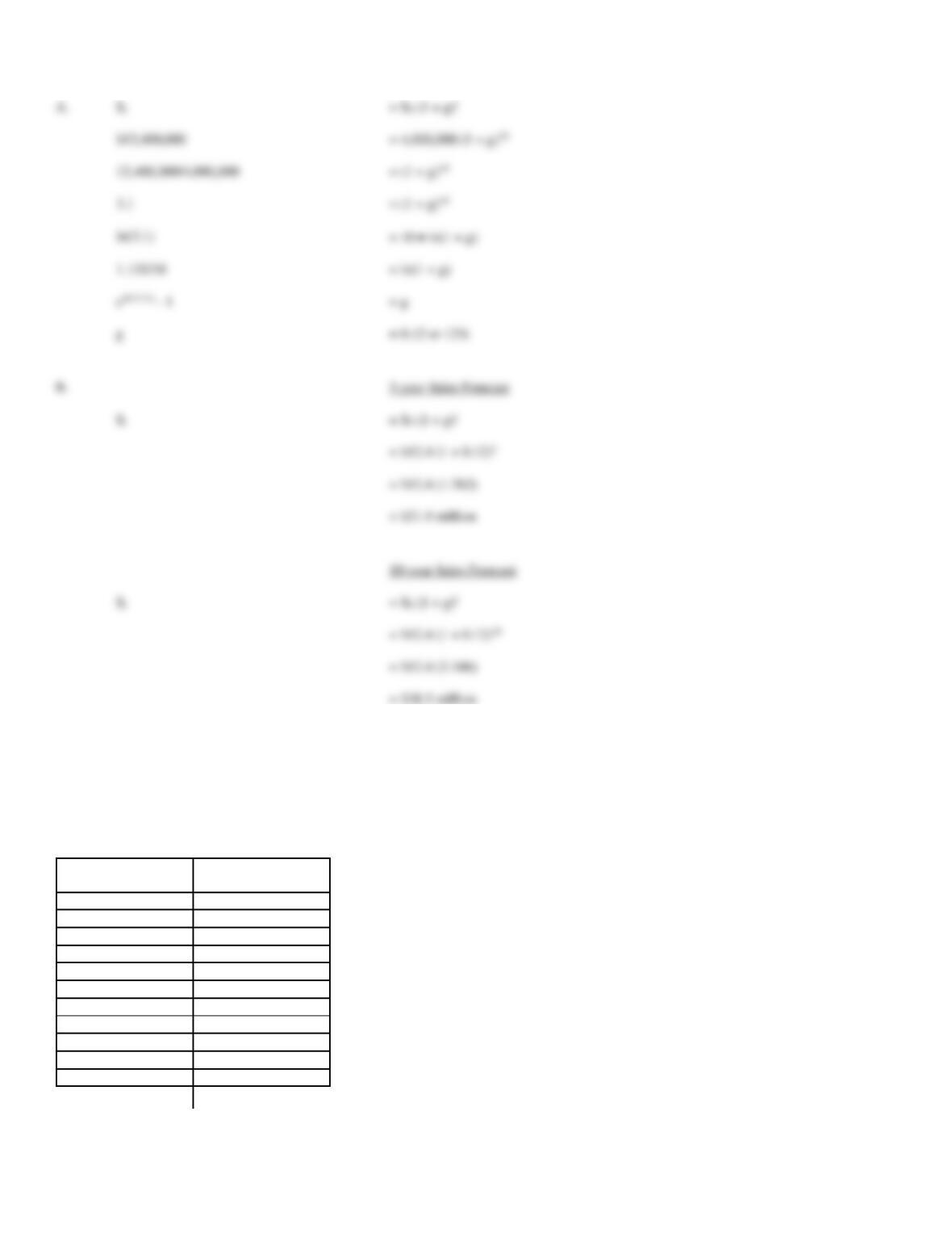
28. Annual Compounding. The following table shows annual sales data for Stuff Happens, Inc., over the
ten-year 1998-2008 period:
Year
Sales
($ Millions)
1998
$2.0
1999
2.2
2000
2.4
2001
2.6
2002
2.8
2003
3.0
2004
3.2
2005
3.5
2006
3.8
2007
4.1
2008
4.3
$12,400,000
12,400,000/4,000,000
3.1
= 10 • ln(1 + g)
1.131/10
= ln(1 + g)
= g
g
= 0.12 or 12%
5-year Sales Forecast
= $12.4 (1.762)
= $21.9 million
= $12.4 (3.106)
= $38.5 million
A.
Calculate the 1998-2008 growth rate in sales using the constant rate of change model with annual compounding.
B.
Forecast sales for the years 2011 and 2013.
A.
$4,300,000
4,300,000/2,000,000
2.15
= 10 • ln(1 + g)
0.765/10
= ln(1 + g)
= g
g
= 0.08 or 8%
2011 Sales Forecast
= $4.3 (1.300)
= $5.4 million
2013 Sales Forecast
= $4.3 (1.469)
= $6.3 million
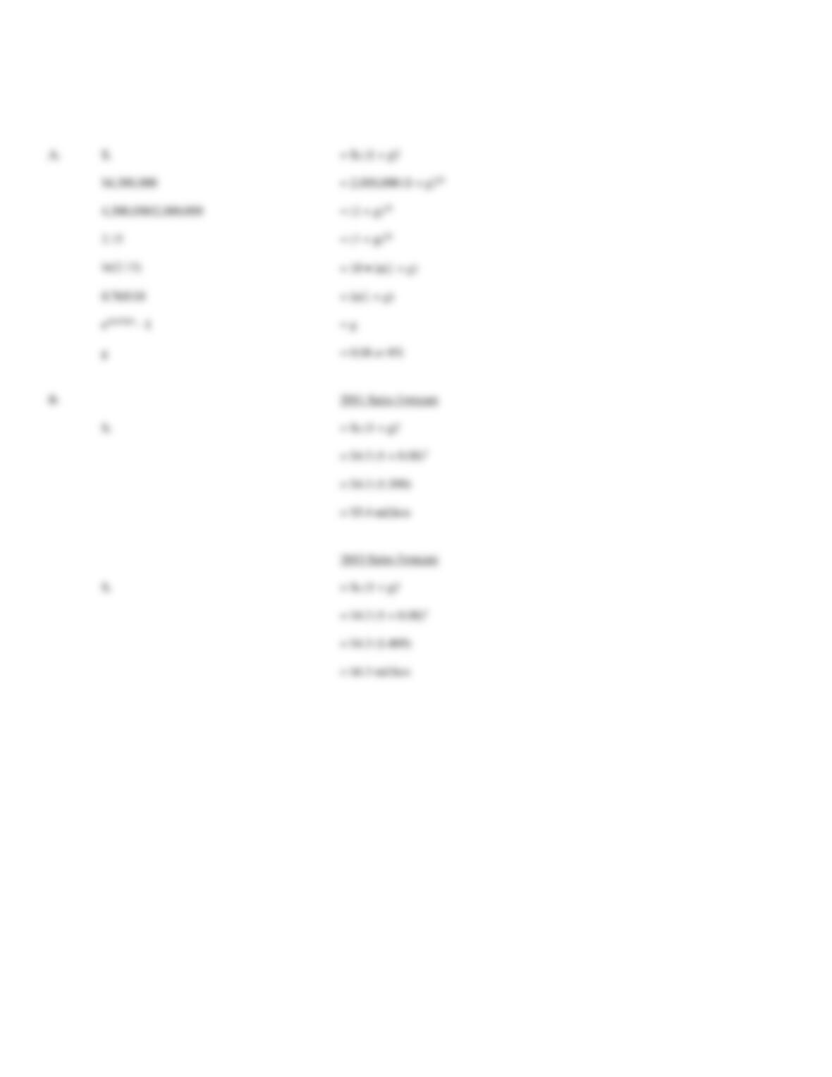
29. Annual Compounding. The following table shows annual sales data for Security Watch, Inc., over the
ten-year 1998-2008 period:
Year
Sales
($ Thousands)
1998
$100
1999
150
2000
200
2001
220
2002
280
2003
360
2004
480
2005
500
2006
540
2007
580
2008
620
A.
Calculate the 1998-2008 growth rate in sales using the constant rate of change model with annual compounding.
B.
Forecast sales for the years 2011 and 2016.
A.
$620
620/100
6.2
= 10 • ln(1 + g)
1.824/10
= ln(1 + g)
= g
g
= 0.2 or 20%
B.
2011 Sales Forecast
= $620 (1.728)
= $1,071.4 thousand
2016 Sales Forecast
30. Continuous Compounding. Nicholas Nickelby, a quality control supervisor for Vinyl Windows, Inc., is
concerned about an increase in distribution costs per unit from $10 to $13.80 over the last four years. Nickelby
feels that setting up a new direct-sales distribution network at a cost of $17.50 per unit may soon be desirable.
A.
Calculate the unit cost growth rate using the constant rate of change model with continuous compounding.
B.
Forecast when unit distribution costs will exceed the current cost of direct-sales distribution.
31. Continuous Compounding. Elizabeth Corday, a quality control supervisor for Surgery Products, Inc., is
concerned about an increase in distribution costs for disposable syringes from $40 to $50 per case over the last
five years. Corday feels that setting up a new direct-sales distribution network at a cost of $58.50 per unit may
soon be desirable.
A.
Calculate the unit cost growth rate using the constant rate of change model with continuous compounding.
B.
Forecast when unit distribution costs will exceed the current cost of direct-sales distribution.
$13.80
1.38
g
= 0.32/4
= 0.08 or 8%
B.
Direct-sales cost
$17.50
17.5/13.8
1.27
ln(1.27)
= 0.08t
t
= 0.24/0.08
= 3 years

32. Continuous Compounding. Mark Greene, a control supervisor for County General, Inc., is concerned
about an increase in distribution costs per unit from $24.50 to $25 over the last four years. Greene feels that
setting up a new direct-sales distribution network at a cost of $27.50 per unit may soon be desirable.
A.
Calculate the unit cost growth rate using the constant rate of change model with continuous compounding.
B.
Forecast when unit distribution costs will exceed the current cost of direct-sales distribution.
A.
50/40
ln(1.25)
= 5g
= 0.04 or 4%
$58.50
1.17
t
= 0.16/0.04
33. Continuous Compounding. Abby Lockheart, a quality control supervisor for Intensive care, Inc., is
concerned about an increase in distribution costs per unit from $3 to $3.27 over the last three years. Lockheart
feels that setting up a new direct-sales distribution network at a cost of $3.56 per unit may soon be desirable.
A.
Calculate the unit cost growth rate using the constant rate of change model with continuous compounding.
B.
Forecast when unit distribution costs will exceed the current cost of direct-sales distribution.
A.
ln(1.02)
= 4g
= 0.05 or 5%
$27.50
1.10
t
= 0.10/0.05
34. Sales Forecast Modeling. The change in the quantity of product A demanded in any given week is
inversely proportional to the change in sales of product B in the previous week. That is, if sales of B rose by X
percent last week, sales of A can be expected to fall by X percent this week.
A.
Write the equation for next week’s sales of A, using the symbols A = sales of Product A, B = sales of Product B, and t = time. Assume
there will be no shortages of either product.
B.
Last week 500 units of A and 250 units of B were sold. Two weeks ago, 200 units of Product B were sold. What would you predict the
sales of A to be this week?
35. Sales Forecast Modeling. The change in the quantity of Beta service demanded in any given week is
inversely proportional to the change in sales by Alpha in the previous week. That is, if sales of Alpha rose by X
percent last week, sales of Beta can be expected to fall by 0.5X percent this week.
A.
Write the equation for next week’s sales of Beta, using the symbols B = sales of Beta services, A = Alpha sales, and t = time. Assume
there will be no shortages of either product.
B.
Last week 200 units of Beta and 450 units of Alpha were sold. Two weeks ago, 300 units of Alpha were sold. What would you predict
the sales of Beta to be this week?
36. Sales Forecast Modeling. The change in the quantity of Cheez Sticks demanded in any given week is
inversely proportional to the change in sales of Pretzel Q’s in the previous week. That is, if sales of Pretzel Q’s
fell by X percent last week, sales of Cheez Sticks can be expected to rise by 2X percent this week.
A.
Write the equation for next week’s sales of Cheez Sticks, using the symbols C = sales of Cheez Sticks, Q = sales of Pretzel Q‘s, and t =
time. Assume there will be no shortages of either product.
B.
Last week 600 units of C and 350 units of Q were sold. Two weeks ago, 400 units of Q were sold. What would you predict the sales of
C to be this week?
37. Sales Forecast Modeling. The change in the quantity of product C demanded in any given week is
inversely proportional to the change in sales of product D in the previous week. That is, if sales of D rose by X
percent last week, sales of C can be expected to fall by X percent this week.
A.
Write the equation for next week’s sales of C, using the symbols C = sales of product C, D = sales of product D, and t = time. Assume
there will be no shortages of either product.
B.
Last week 750 units of C and 600 units of D were sold. Two weeks ago, 500 units of product D were sold. What would you predict the
sales of C to be this week?