44. Demand Estimation. The Wallpaper Shop, Inc., is a rapidly growing chain of wallpaper shops that caters to
the do-it-yourself home remodeling market. During the past year, 15 stores were operated in small to
medium-size metropolitan markets. An in-house study of sales by these outlets revealed the following (standard
errors in parentheses):
Q
= -11,000 – 50P + 25PX + 0.5A + 0.1I + 500GR
(9,000) (20) (2.5) (0.3) (0.06) (200)
R2
= 90%
Standard Error of the Estimate = 800.
Here, Q is the number of customers served, P is the average price per customer, PX is the average cost of professionally wallpapering a small room, A
is advertising expenditures (in dollars), I is disposable income per capita (in dollars), and GR is the rate of population growth per year (in percent).
A.
Fully evaluate and interpret these empirical results on an overall basis.
B.
Is quantity demanded sensitive to “own” price?
C.
Davis, California, is a typical market covered by this analysis. During the past year in the Davis market, P = $50, PX = $100, A =
$50,000, I = $100,000 and GR = 2%. Calculate and interpret the relevant advertising point elasticity.
D.
Assume that the preceding model and data are relevant for the coming period. Estimate the probability that the Davis store will make a
profit during the coming year if total costs are projected to be $1.25 million.
(i)
(iv)
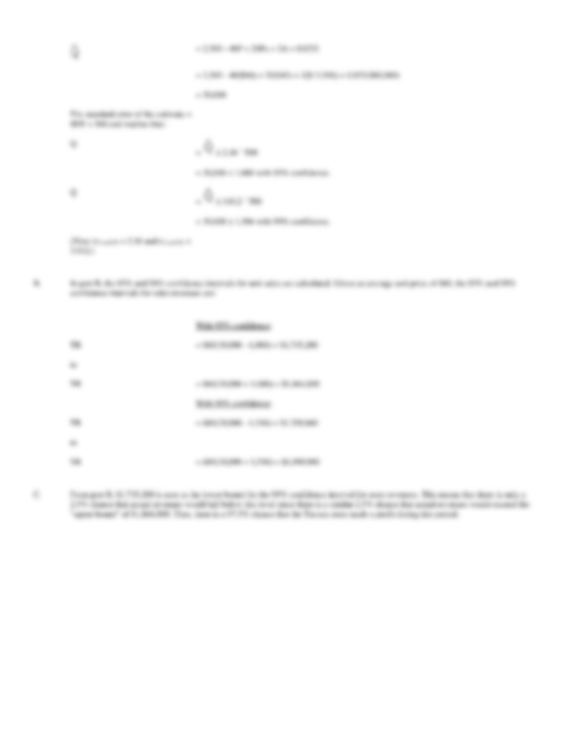
Standard error of the estimate = SEE = 800 implying that
= 2.262 ´ 800 with 95% confidence.
= 3.25 ´ 800 with 99% confidence.
where,
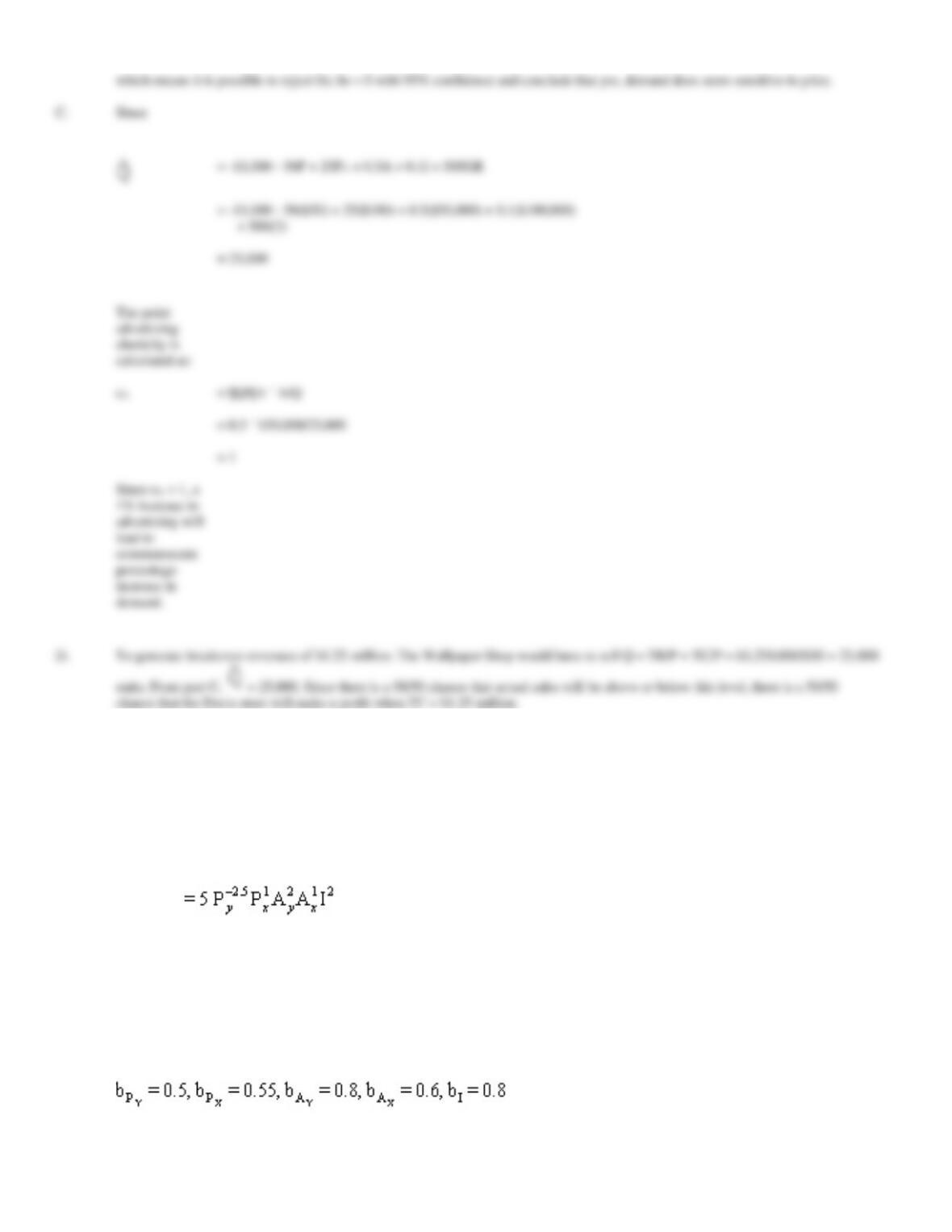
45. Elasticity Estimation. Breakaway Tours, Inc., has estimated the following multiplicative demand function
for packaged holiday tours in the Flushing, New York, market using quarterly data covering the past five years
(20 observations):
Qy
R2
= 0.90
Standard Error of the Estimate = 10.
Here, Qy is the quantity of tours sold, Py is average tour price, Px is average price for some other good, Ay is tour advertising, Ax is advertising of
some other good, and I is per capita disposable income. The standard errors of the exponents in the preceding multiplicative demand function are
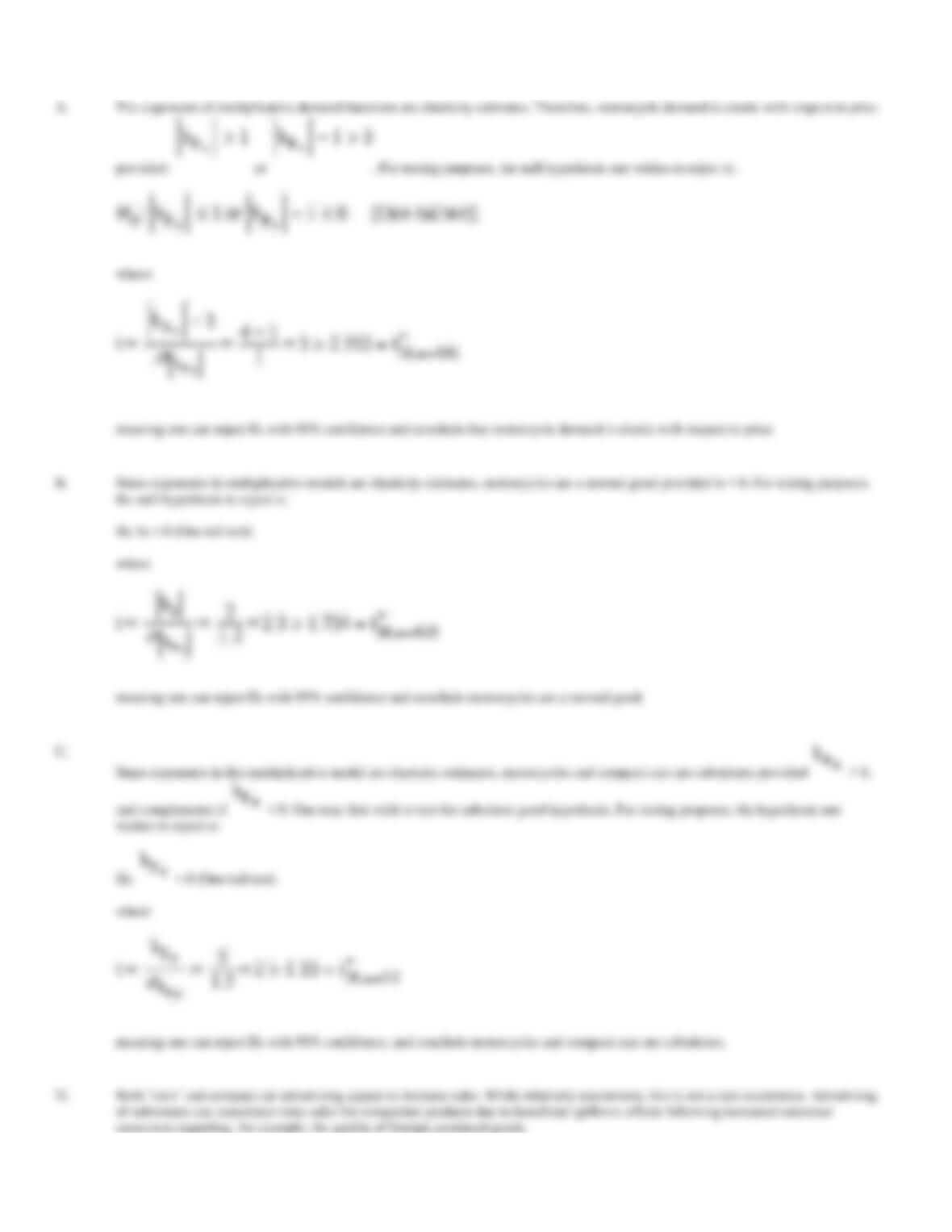
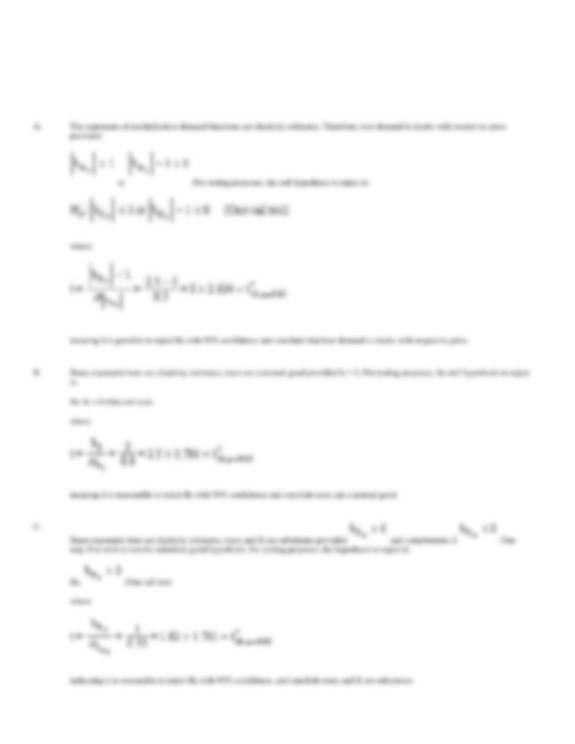
which means it is possible to reject H0: bP = 0 with 95% confidence and conclude that yes, demand does seem sensitive to price.
Since
+ 500(2)
= 25,000
= 0.5 ´ $50,000/25,000
= 1
A.
Is tour demand elastic with respect to price?
B.
Are tours a normal good?
C.
Is X a complement good or substitute good?
D.
Given your answer to part C, can you explain why the demand effects of Ay and Ax are both positive?
where:
meaning it is possible to reject H0 with 99% confidence and conclude that tour demand is elastic with respect to price.
where
meaning it is reasonable to reject H0 with 95% confidence and conclude tours are a normal good.
may first wish to test the substitute good hypothesis. For testing purposes, the hypothesis to reject is:
where
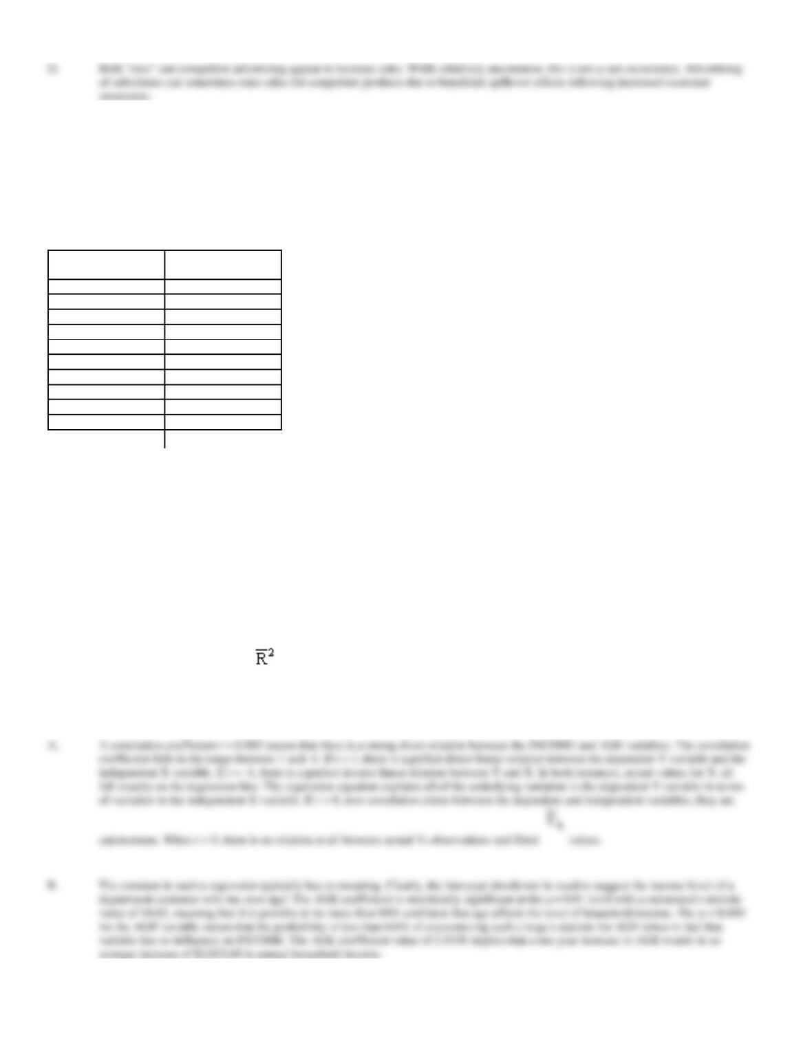
46. Correlation and Simple Regression. Market Analysis, Inc., has conducted a survey to learn the income
characteristics of an N = 10 sample of department store customers. The survey asked each customer his or her
age and household annual income. Survey results were as follows
Household Income
(000)
Respondent Age
$138
43
123
35
137
42
136
42
129
40
123
37
140
43
112
30
116
31
115
33
A.
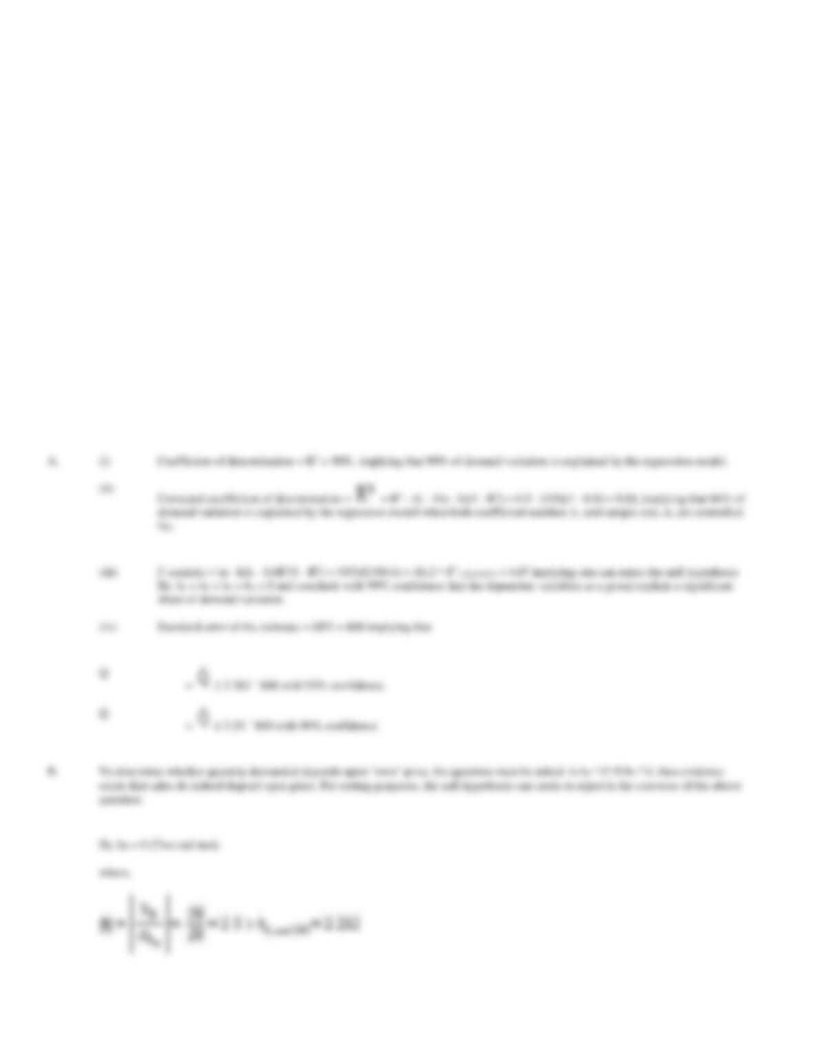
Interpret the coefficient of correlation between the INCOME and AGE variables of 0.982.
B.
Interpret the following results for a simple regression over this sample where INCOME is the dependent Y variable and AGE is the
independent X variable:
The regression equation is:
INCOME = 50.4 + 2.03 AGE
Predictor
Coef
Stdev
t-ratio
p
Constant
50.438
5.263
9.58
0.000
AGE
2.0336
0.1388
14.65
0.000
SEE = 2.117
R2 = 96.4%
= 96.0%
F = 214.53 (p = 0.000)
autonomous. When r = 0, there is no relation at all between actual Yt observations and fitted values.
average increase of $2,033.60 in annual household income.

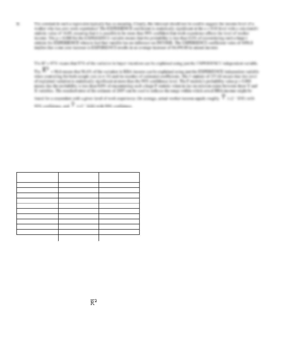
47. Correlation and Simple Regression. Test Markets, Inc., has conducted a survey to learn the income
characteristics of an n = 10 sample of construction workers. The survey asked worker his or her annual income
and number of years work experience. Survey results are:
Income
Years Work
Experience
$25,700
2.5
38,500
6.3
19,700
1.7
19,800
1.8
40,900
6.0
35,600
5.3
45,700
7.0
37,700
4.7
52,100
8.6
27,100
2.7
A.
Interpret the coefficient of correlation between the INCOME and EXPERIENCE variables of 0.985.
B.
Interpret the following results for a simple regression over this sample where INCOME is the dependent Y variable and EXPERIENCE
is the independent X variable:
The regression equation is:
INCOME = 13325 + 4497 EXPERIENCE
Predictor
Coef
Stdev
t ratio
p
Constant
13325
1452
9.18
0.000
EXPERIENCE
4496.8
280.1
16.05
0.000
SEE = 2007
R2 = 97.0%
= 96.6%
variables; they are autonomous. When r = 0, there is no relation at all between actual Yt observations and fitted values.
and (3 ´ SEE) with 99% confidence.
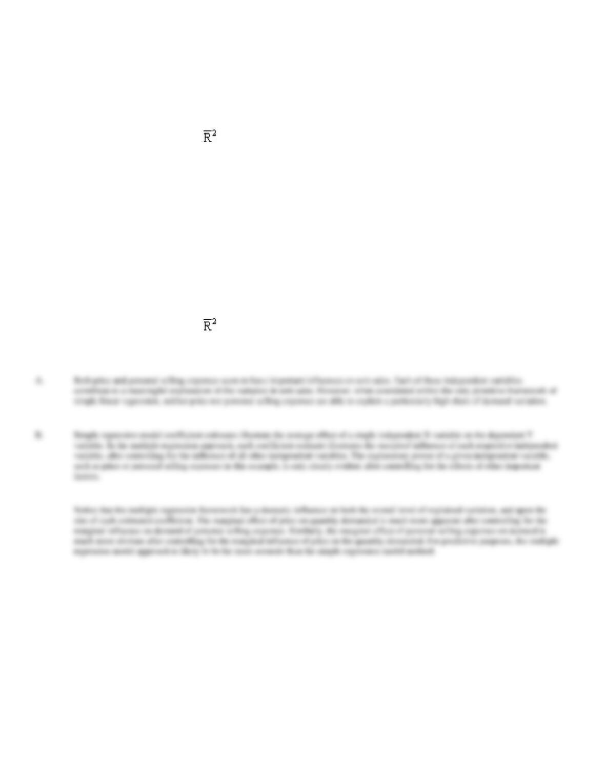
48. Multiple Regression. Kitchen Products, Ltd., is a regional distributor of Regal Bread Making Machine. The
company wishes to assess the relative importance of price reductions versus an increase in personal selling
efforts as means for enhancing product promotion. To this end, the company recently used a regression analysis
approach to study the following monthly unit sales, price, and personal selling expense information for the
Bozeman, Montana market:
Unit Sales
Price
Personal Selling
Expenses
132
$74
$1,140
203
74
1,400
217
55
1,160
255
53
1,210
252
64
1,490
239
70
1,460
152
75
1,200
197
58
1,020
230
65
1,390
154
61
1,040
As a first step in the analysis, the company ran simple regressions of unit sales on each of the potentially important independent variables of price and
personal selling expenses:
The first simple regression equation is:
SALES = 371 – 2.59 PRICE
Predictor
Coef
Stdev
t ratio
p
Constant
371.0
109.5
3.39
0.010
PRICE
-2.587
1.676
-1.54
0.161
SEE = 40.94
R2 = 22.9%
= 13.3%
The second simple regression equation is:
SALES = 5.9 + 0.158 SELLEXP
Predictor
Coef
Stdev
t ratio
p
Constant
5.89
90.10
0.07
0.949
SELLEXP
0.15764
0.07142
2.21
0.058
SEE = 36.77
R2 = 37.8%
= 30.1%
A.
Based on these simple regression model results, do either of the potentially important independent variables affect unit sales?
B.
Characterize the differences between each simple regression model coefficient estimate from part A with those estimated using the
following multiple regression:
The multiple regression equation is:
SALES = 195 – 4.33 PRICE + 0.231 SELLEXP
Predictor
Coef
Stdev
t ratio
p
Constant
194.92
38.27
5.09
0.000
PRICE
-4.3296
0.5396
-8.02
0.000
SELLEXP
0.23115
0.02560
9.03
0.000
SEE = 12.31
R2 = 93.9%
= 92.2%
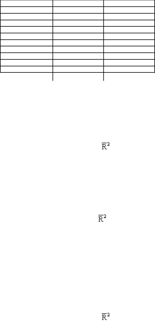
49. Multiple Regression. Maastrict Controls, Ltd., is a regional producer of sophisticated precision control
devices. To assess the potential payoff to adopting the recommendations of a Total Quality Management (TQM)
seminar attended by managerial staff, the company has decided to analyze the sales effects of price and product
quality for a range of leading products. The company recently compiled and used a regression analysis approach
to study the following unit sales, price, and product quality information:
Unit Sales
Price
Percent Failure
33,500
$4.40
4.09%
92,600
4.79
3.56
32,400
4.08
4.15
81,700
3.47
4.18
144,800
2.06
4.33
114,300
3.74
3.58
156,600
3.11
3.75
158,000
2.29
3.95
58,100
3.24
4.39
135,000
2.10
4.45
As a first step in the analysis, the company ran simple regressions of unit sales on each of the potentially important independent variables of price and
the percent failure rate (product quality):
SALES = 220440 – 35980 PRICE
Predictor
Coef
Stdev
t ratio
p
Constant
220440
43214
5.10
0.000
PRICE
-35980
12525
-2.87
0.021
SEE = 36063
R2 = 50.8%
= 44.6%
The second simple regression equation is:
SALES = 74997 + 26858 FAILURE
Predictor
Coef
Stdev
t ratio
p
Constant
74997
52336
1.43
0.190
FAILURE
26858
52073
0.52
0.620
SEE = 50567
R2 = 3.2%
= 0.0%
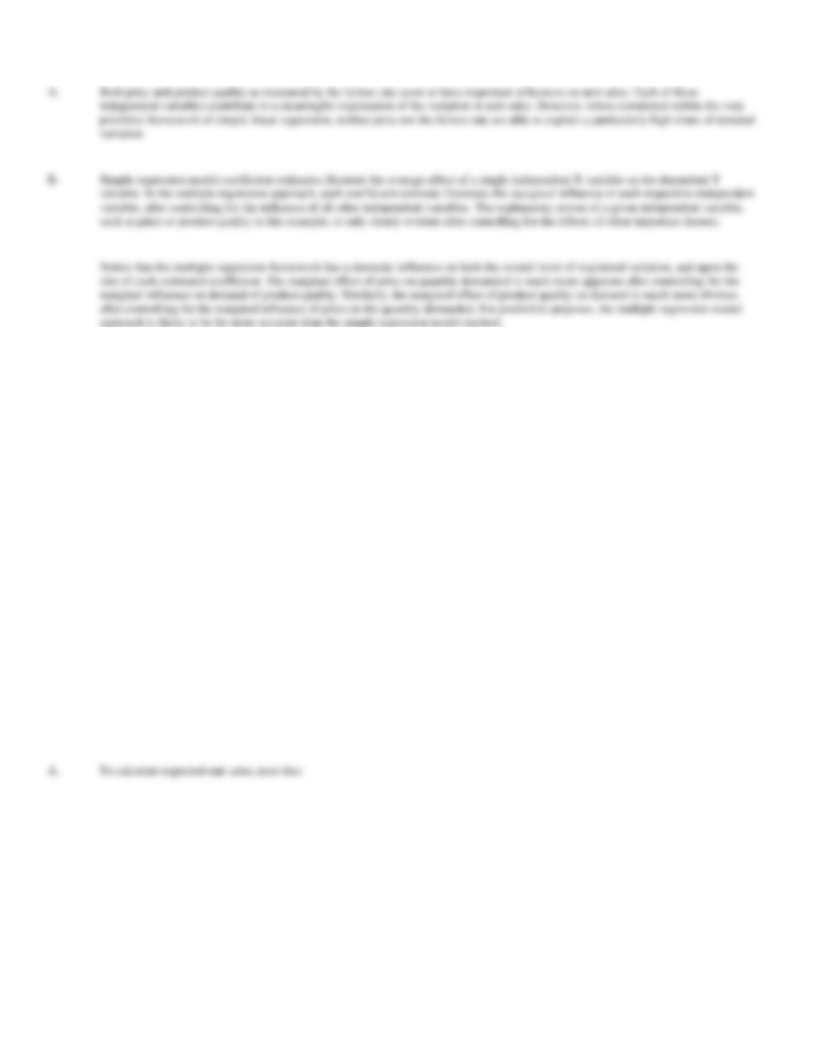
A.
Based on these simple regression model results, do either of the potentially important independent variables affect unit sales?
B.
Characterize the differences between each simple regression model coefficient estimate from part A with those estimated using the
following multiple regression:
SALES = 178434 – 56659 PRICE + 115808 FAILURE
Predictor
Coef
Stdev
t ratio
p
Constant
178434
17414
10.25
0.000
PRICE
-56659
5584
-10.15
0.000
FAILURE
115808
16558
6.99
0.000
SEE = 13641
R2 = 93.8%
= 92.1%
50. Profit Probability Estimation. Intimate Lighting, Inc., is a rapidly growing lighting accessory outlets that
caters to the do-it-yourself home remodeling market. During the past year, 18 stores were operated in small to
medium-size metropolitan markets. An in-house study of sales by these outlets revealed the following (standard
errors in parentheses):
Q
= 2,500 – 40P + 20PX + 2A + 0.25I
(1,500) (20) (15) (1.3) (0.01)
R2
= 86%
Standard Error of the Estimate = 500.
Here, Q is unit sales, P is unit price, PX is the average unit price at competitor stores, A is advertising expenditures, and I is income per capita.
A.
Tucson, Arizona was a typical market covered by this analysis. In the Tucson market, “own” price was $60, competitor price was $45,
advertising was $13,500, and income was an average $80,000. Calculate and interpret the expected level of unit sales, as well as the
95% and 99% confidence regions for actual sales.
B.
Calculate the 95% and 99% confidence regions for actual revenues in the Tucson market.
C.
Estimate the probability that the Tucson store made a profit during this period if total costs were $1,735,200.
To calculate expected unit sales, note that:
such as price or product quality in this example, is only clearly evident after controlling for the effects of other important factors.