
Introduction to Econometrics, 3e (Stock)
Chapter 5 Regression with a Single Regressor: Hypothesis Tests and Confidence
Intervals
5.1 Multiple Choice
1) Heteroskedasticity means that
A) homogeneity cannot be assumed automatically for the model.
B) the variance of the error term is not constant.
C) the observed units have different preferences.
D) agents are not all rational.
2) With heteroskedastic errors, the weighted least squares estimator is BLUE. You should use OLS with
heteroskedasticity–robust standard errors because
A) this method is simpler.
B) the exact form of the conditional variance is rarely known.
C) the Gauss–Markov theorem holds.
D) your spreadsheet program does not have a command for weighted least squares.
3) When estimating a demand function for a good where quantity demanded is a linear function of the
price, you should
A) not include an intercept because the price of the good is never zero.
B) use a one–sided alternative hypothesis to check the influence of price on quantity.
C) use a two–sided alternative hypothesis to check the influence of price on quantity.
D) reject the idea that price determines demand unless the coefficient is at least 1.96.
4) The t–statistic is calculated by dividing
A) the OLS estimator by its standard error.
B) the slope by the standard deviation of the explanatory variable.
C) the estimator minus its hypothesized value by the standard error of the estimator.
D) the slope by 1.96.
5) The confidence interval for the sample regression function slope
A) can be used to conduct a test about a hypothesized population regression function slope.
B) can be used to compare the value of the slope relative to that of the intercept.
C) adds and subtracts 1.96 from the slope.
D) allows you to make statements about the economic importance of your estimate.

6) If the absolute value of your calculated t–statistic exceeds the critical value from the standard normal
distribution, you can
A) reject the null hypothesis.
B) safely assume that your regression results are significant.
C) reject the assumption that the error terms are homoskedastic.
D) conclude that most of the actual values are very close to the regression line.
7) Under the least squares assumptions (zero conditional mean for the error term, Xi and Yi being i.i.d.,
and Xi and ui having finite fourth moments), the OLS estimator for the slope and intercept
A) has an exact normal distribution for n > 15.
B) is BLUE.
C) has a normal distribution even in small samples.
D) is unbiased.
8) In general, the t–statistic has the following form:
A)
estimate–hypothesize value
standard error of estimate
B)
estimator
standard error of estimate
C)
estimator-hypothesize value
standard error of estimate
D)
n
estimator oferror standard
valueehypothesiz–estimator
9) Consider the following regression line: = 698.9 – 2.28 × STR. You are told that the t–statistic on
the slope coefficient is 4.38. What is the standard error of the slope coefficient?
A) 0.52
B) 1.96
C) –1.96
D) 4.38
10) Imagine that you were told that the t–statistic for the slope coefficient of the regression line =
698.9 – 2.28 × STR was 4.38. What are the units of measurement for the t–statistic?
A) points of the test score
B) number of students per teacher
C)
TestScore
STR
D) standard deviations

11) The construction of the t–statistic for a one– and a two–sided hypothesis
A) depends on the critical value from the appropriate distribution.
B) is the same.
C) is different since the critical value must be 1.645 for the one–sided hypothesis, but 1.96 for the two–
sided hypothesis (using a 5% probability for the Type I error).
D) uses ±1.96 for the two–sided test, but only +1.96 for the one–sided test.
12) The p–value for a one–sided left–tail test is given by
A) Pr(Z – tact ) = φ(tact).
B) Pr(Z < tact ) = φ(tact).
C) Pr(Z < tact ) < 1.645.
D) cannot be calculated, since probabilities must always be positive.
13) The 95% confidence interval for β1 is the interval
A) (β1 – 1.96SE)(β1), β1 + 1.96SE(β1)).
B) ( 1 – 1.645SE)( 1), 1 + 1.645SE(1)).
C) ( 1 – 1.96SE)( 1), 1 + 1.96SE(1)).
D) ( 1 – 1.96, 1 + 1.96).
14) The 95% confidence interval for β0 is the interval
A) (β0 – 1.96SE(β0), β0 + 1.96SE(β0)).
B) (β0 – 1.645SE(0), 0 + 1.645SE(0)).
C) ( 0 – 1.96SE(0), 0 + 1.96SE(0)).
D) ( 0 – 1.96, 0 + 1.96).
15) The 95% confidence interval for the predicted effect of a general change in X is
A) (β1△x – 1.96SE(β1) × △x, β1△x + 1.96SE(β1) × △x).
B) ( 1△x – 1.645SE(1) × △x, 1△x + 1.645SE(1) × △x).
C) ( 1△x – 1.96SE(1) × △x, 1△x + 1.96SE(1) × △x).
D) ( 1△x – 1.96, 1△x + 1.96).
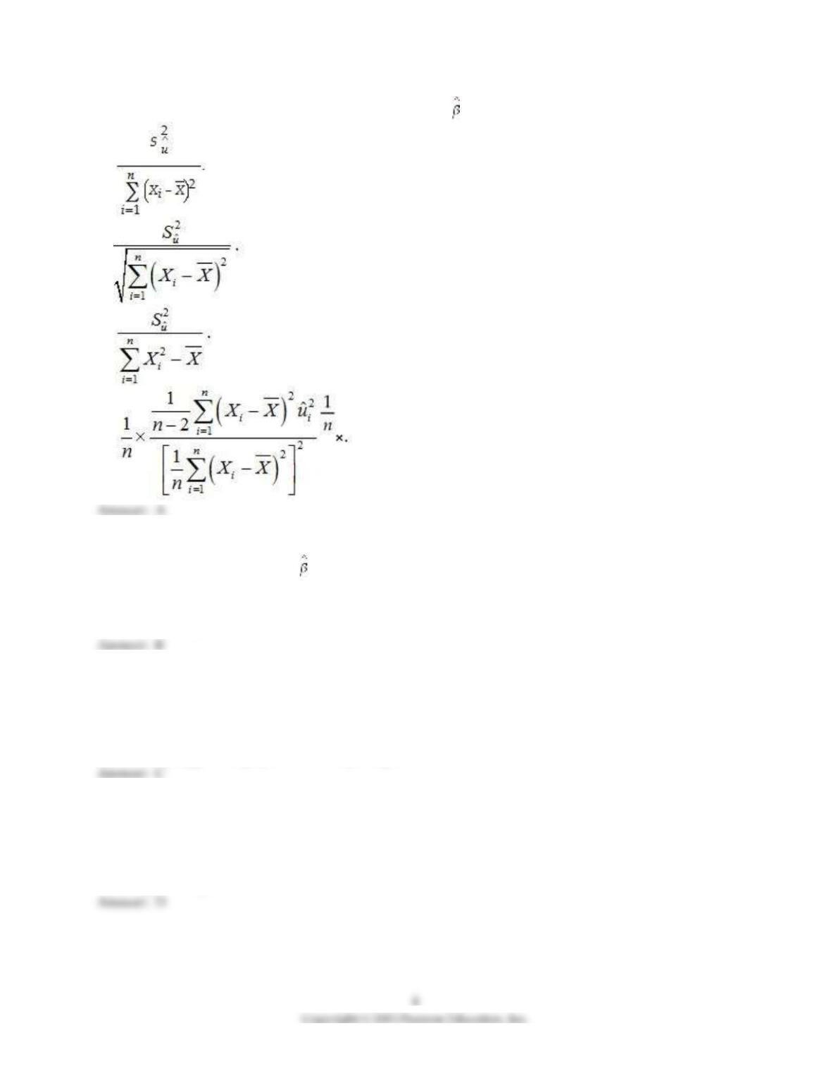
16) The homoskedasticity–only estimator of the variance of 1 is
A)
B)
C)
D)
17) One of the following steps is not required as a step to test for the null hypothesis:
A) compute the standard error of 1.
B) test for the errors to be normally distributed.
C) compute the t–statistic.
D) compute the p–value.
18) Finding a small value of the p–value (e.g. less than 5%)
A) indicates evidence in favor of the null hypothesis.
B) implies that the t–statistic is less than 1.96.
C) indicates evidence in against the null hypothesis.
D) will only happen roughly one in twenty samples.
19) The only difference between a one– and two–sided hypothesis test is
A) the null hypothesis.
B) dependent on the sample size n.
C) the sign of the slope coefficient.
D) how you interpret the t–statistic.
20) A binary variable is often called a
A) dummy variable.
B) dependent variable.
C) residual.
D) power of a test.
21) The error term is homoskedastic if
A) var(uiis constant for i = 1,…, n.
B) var(uidepends on x.
C) Xi is normally distributed.
D) there are no outliers.
22) In the presence of heteroskedasticity, and assuming that the usual least squares assumptions hold, the
OLS estimator is
A) efficient.
B) BLUE.
C) unbiased and consistent.
D) unbiased but not consistent.
23) The proof that OLS is BLUE requires all of the following assumptions with the exception of:
A) the errors are homoskedastic.
B) the errors are normally distributed.
C) E(ui.
D) large outliers are unlikely.
24) If the errors are heteroskedastic, then
A) OLS is BLUE.
B) WLS is BLUE if the conditional variance of the errors is known up to a constant factor of
proportionality.
C) LAD is BLUE if the conditional variance of the errors is known up to a constant factor of
proportionality.
D) OLS is efficient.
25) The homoskedastic normal regression assumptions are all of the following with the exception of:
A) the errors are homoskedastic.
B) the errors are normally distributed.
C) there are no outliers.
D) there are at least 10 observations.

26) Using the textbook example of 420 California school districts and the regression of testscores on the
student–teacher ratio, you find that the standard error on the slope coefficient is 0.51 when using the
heteroskedasticity robust formula, while it is 0.48 when employing the homoskedasticity only formula.
When calculating the t–statistic, the recommended procedure is to
A) use the homoskedasticity only formula because the t–statistic becomes larger
B) first test for homoskedasticity of the errors and then make a decision
C) use the heteroskedasticity robust formula
D) make a decision depending on how much different the estimate of the slope is under the two
procedures
27) Consider the estimated equation from your textbook
=698.9 – 2.28 STR, R2 = 0.051, SER = 18.6
(10.4) (0.52)
The t–statistic for the slope is approximately
A) 4.38
B) 67.20
C) 0.52
D) 1.76
28) You have collected data for the 50 U.S. states and estimated the following relationship between the
change in the unemployment rate from the previous year ( ) and the growth rate of the respective
state real GDP (gy). The results are as follows
= 2.81 — 0.23 gy, R2= 0.36, SER = 0.78
(0.12) (0.04)
Assuming that the estimator has a normal distribution, the 95% confidence interval for the slope is
approximately the interval
A) [2.57, 3.05]
B) [–0.31,0.15]
C) [–0.31, –0.15]
D) [–0.33, –0.13]
29) Using 143 observations, assume that you had estimated a simple regression function and that your
estimate for the slope was 0.04, with a standard error of 0.01. You want to test whether or not the estimate
is statistically significant. Which of the following possible decisions is the only correct one:
A) you decide that the coefficient is small and hence most likely is zero in the population
B) the slope is statistically significant since it is four standard errors away from zero
C) the response of Y given a change in X must be economically important since it is statistically
significant
D) since the slope is very small, so must be the regression R2.
30) You extract approximately 5,000 observations from the Current Population Survey (CPS) and estimate
the following regression function:
= 3.32 — 0.45 Age, R2= 0.02, SER = 8.66
(1.00) (0.04)
where ahe is average hourly earnings, and Age is the individual’s age. Given the specification, your 95%
confidence interval for the effect of changing age by 5 years is approximately
A) [$1.96, $2.54]
B) [$2.32, $4.32]
C) [$1.35, $5.30]
D) cannot be determined given the information provided
5.2 Essays and Longer Questions
1) (Continuation from Chapter 4) Sir Francis Galton, a cousin of James Darwin, examined the
relationship between the height of children and their parents towards the end of the 19th century. It is
from this study that the name “regression” originated. You decide to update his findings by collecting
data from 110 college students, and estimate the following relationship:
= 19.6 + 0.73 × Midparh, R2 = 0.45, SER = 2.0
(7.2) (0.10)
where Studenth is the height of students in inches, and Midparh is the average of the parental heights.
Values in parentheses are heteroskedasticity robust standard errors. (Following Galton’s methodology,
both variables were adjusted so that the average female height was equal to the average male height.)
(a) Test for the statistical significance of the slope coefficient.
(b) If children, on average, were expected to be of the same height as their parents, then this would imply
two hypotheses, one for the slope and one for the intercept.
(i) What should the null hypothesis be for the intercept? Calculate the relevant t–statistic and carry out the
hypothesis test at the 1% level.
(ii) What should the null hypothesis be for the slope? Calculate the relevant t–statistic and carry out the
hypothesis test at the 5% level.
(c) Can you reject the null hypothesis that the regression R2 is zero?
(d) Construct a 95% confidence interval for a one inch increase in the average of parental height.
2) (Requires Appendix) (Continuation from Chapter 4) At a recent county fair, you observed that at one
stand people’s weight was forecasted, and were surprised by the accuracy (within a range). Thinking
about how the person could have predicted your weight fairly accurately (despite the fact that she did
not know about your “heavy bones”), you think about how this could have been accomplished. You
remember that medical charts for children contain 5%, 25%, 50%, 75% and 95% lines for a weight/height
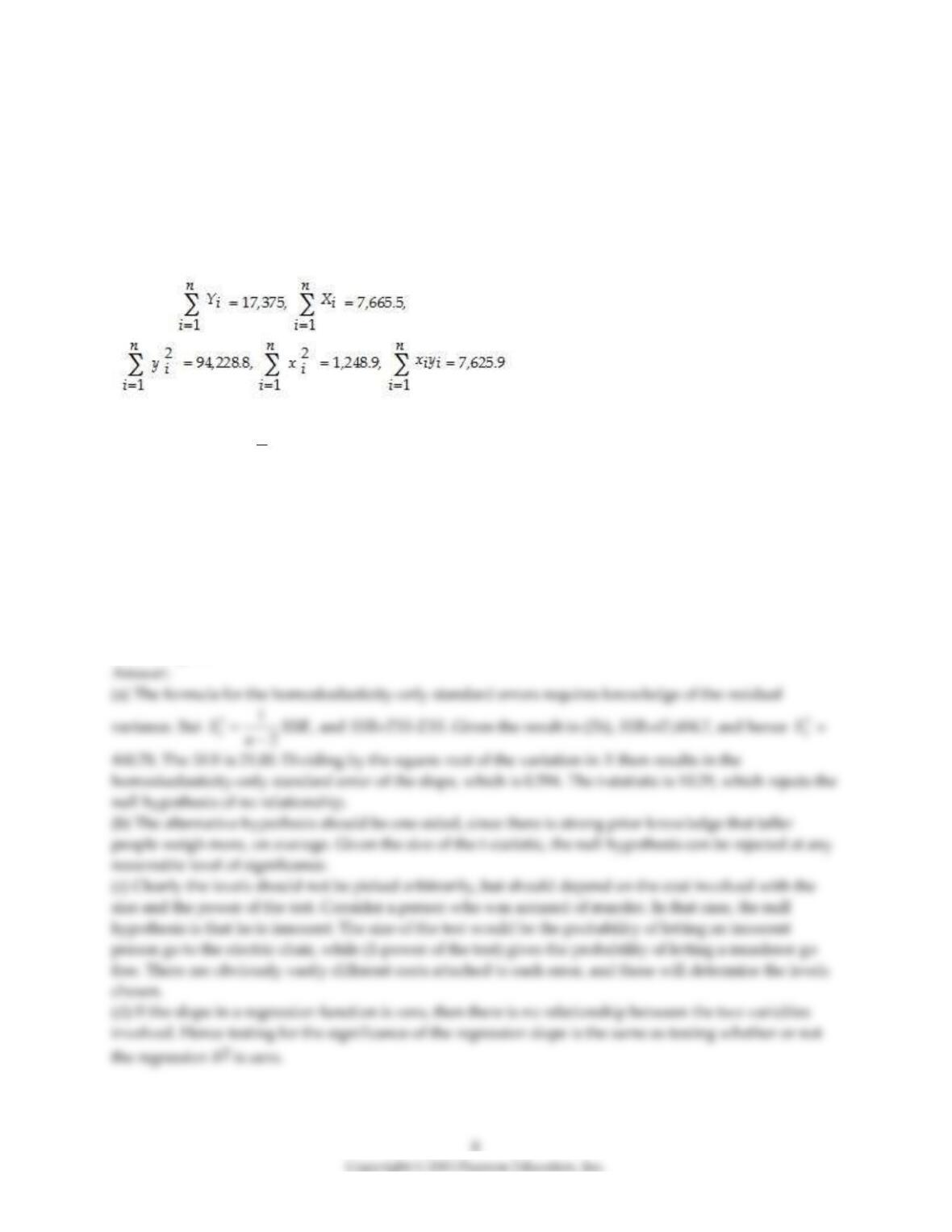
relationship and decide to conduct an experiment with 110 of your peers. You collect the data and
calculate the following sums:
where the height is measured in inches and weight in pounds. (Small letters refer to deviations from
means as in zi = Zi –
Z
.)
(a) Calculate the homoskedasticity–only standard errors and, using the resulting t–statistic, perform a test
on the null hypothesis that there is no relationship between height and weight in the population of
college students.
(b) What is the alternative hypothesis in the above test, and what level of significance did you choose?
(c) Statistics and econometrics textbooks often ask you to calculate critical values based on some level of
significance, say 1%, 5%, or 10%. What sort of criteria do you think should play a role in determining
which level of significance to choose?
(d) What do you think the relationship is between testing for the significance of the slope and whether or
not the regression R2 is zero?
3) You have obtained measurements of height in inches of 29 female and 81 male students (Studenth) at
your university. A regression of the height on a constant and a binary variable (BFemme), which takes a
value of one for females and is zero otherwise, yields the following result:
= 71.0 – 4.84×BFemme , R2 = 0.40, SER = 2.0
(0.3) (0.57)
(a) What is the interpretation of the intercept? What is the interpretation of the slope? How tall are
females, on average?
(b) Test the hypothesis that females, on average, are shorter than males, at the 1% level.
(c) Is it likely that the error term is homoskedastic here?
4) (continuation from Chapter 4, number 3) You have obtained a sub–sample of 1744 individuals from the
Current Population Survey (CPS) and are interested in the relationship between weekly earnings and age.
The regression, using heteroskedasticity–robust standard errors, yielded the following result:
= 239.16 + 5.20×Age , R2 = 0.05, SER = 287.21.,
(20.24) (0.57)
where Earn and Age are measured in dollars and years respectively.
(a) Is the relationship between Age and Earn statistically significant?
(b) The variance of the error term and the variance of the dependent variable are related. Given the
distribution of earnings, do you think it is plausible that the distribution of errors is normal?
(c) Construct a 95% confidence interval for both the slope and the intercept.
5) (Continuation from Chapter 4, number 5) You have learned in one of your economics courses that one
of the determinants of per capita income (the “Wealth of Nations”) is the population growth rate.
Furthermore you also found out that the Penn World Tables contain income and population data for 104
countries of the world. To test this theory, you regress the GDP per worker (relative to the United States)
in 1990 (RelPersInc) on the difference between the average population growth rate of that country (n) to
the U.S. average population growth rate (nus ) for the years 1980 to 1990. This results in the following
regression output:
= 0.518 – 18.831×(n – nus), R2=0.522, SER = 0.197
(0.056) (3.177)
(a) Is there any reason to believe that the variance of the error terms is homoskedastic?
(b) Is the relationship statistically significant?
6) You recall from one of your earlier lectures in macroeconomics that the per capita income depends on
the savings rate of the country: those who save more end up with a higher standard of living. To test this
theory, you collect data from the Penn World Tables on GDP per worker relative to the United States
(RelProd) in 1990 and the average investment share of GDP from 1980–1990 (SK), remembering that
investment equals saving. The regression results in the following output:
= –0.08 + 2.44×SK, R2=0.46, SER = 0.21
(0.04) (0.38)
(a) Interpret the regression results carefully.
(b) Calculate the t–statistics to determine whether the two coefficients are significantly different from
zero. Justify the use of a one–sided or two–sided test.
(c) You accidentally forget to use the heteroskedasticity–robust standard errors option in your regression
package and estimate the equation using homoskedasticity–only standard errors. This changes the results
as follows:
= –0.08 + 2.44×SK, R2=0.46, SER = 0.21
(0.04) (0.26)
You are delighted to find that the coefficients have not changed at all and that your results have become
even more significant. Why haven‘t the coefficients changed? Are the results really more significant?
Explain.
(d) Upon reflection you think about the advantages of OLS with and without homoskedasticity–only
standard errors. What are these advantages? Is it likely that the error terms would be heteroskedastic in
this situation?
7) Carefully discuss the advantages of using heteroskedasticity–robust standard errors over standard
errors calculated under the assumption of homoskedasticity. Give at least five examples where it is very
plausible to assume that the errors display heteroskedasticity.
8) (Requires Appendix material from Chapters 4 and 5) Shortly before you are making a group
presentation on the testscore/student–teacher ratio results, you realize that one of your peers forgot to
type all the relevant information on one of your slides. Here is what you see:
= 698.9 – STR, R2 = 0.051, SER = 18.6
(9.47) (0.48)
In addition, your group member explains that he ran the regression in a standard spreadsheet program,
and that, as a result, the standard errors in parenthesis are homoskedasticity–only standard errors.
(a) Find the value for the slope coefficient.
(b) Calculate the t–statistic for the slope and the intercept. Test the hypothesis that the intercept and the
slope are different from zero.
(c) Should you be concerned that your group member only gave you the result for the homoskedasticity–
only standard error formula, instead of using the heteroskedasticity–robust standard errors?

14
9) (Continuation of the Purchasing Power Parity question from Chapter 4) The news–magazine The
Economist regularly publishes data on the so called Big Mac index and exchange rates between countries.
The data for 30 countries from the April 29, 2000 issue is listed below:
Price of Actual Exchange Rate
Country Currency Big Mac per U.S. dollar
Indonesia Rupiah 14,500 7,945
Italy Lira 4,500 2,088
South Korea Won 3,000 1,108
Chile Peso 1,260 514
Spain Peseta 375 179
Hungary Forint 339 279
Japan Yen 294 106
Taiwan Dollar 70 30.6
Thailand Baht 55 38.0
Czech Rep. Crown 54.37 39.1
Russia Ruble 39.50 28.5
Denmark Crown 24.75 8.04
Sweden Crown 24.0 8.84
Mexico Peso 20.9 9.41
France Franc 18.5 7.07
Israel Shekel 14.5 4.05
China Yuan 9.90 8.28
South Africa Rand 9.0 6.72
Switzerland Franc 5.90 1.70
Poland Zloty 5.50 4.30
Germany Mark 4.99 2.11
Malaysia Dollar 4.52 3.80
New Zealand Dollar 3.40 2.01
Singapore Dollar 3.20 1.70
Brazil Real 2.95 1.79
Canada Dollar 2.85 1.47
Australia Dollar 2.59 1.68
Argentina Peso 2.50 1.00
Britain Pound 1.90 0.63
United States Dollar 2.51
The concept of purchasing power parity or PPP (“the idea that similar foreign and domestic goods …
should have the same price in terms of the same currency,” Abel, A. and B. Bernanke, Macroeconomics, 4th
edition, Boston: Addison Wesley, 476) suggests that the ratio of the Big Mac priced in the local currency
to the U.S. dollar price should equal the exchange rate between the two countries.
After entering the data into your spread sheet program, you calculate the predicted exchange rate per
U.S. dollar by dividing the price of a Big Mac in local currency by the U.S. price of a Big Mac ($2.51). To
test for PPP, you regress the actual exchange rate on the predicted exchange rate.
The estimated regression is as follows:
= –27.05 + 1.35 × 1.35×Pr edExRate R2 = 0.994, n = 29, SER = 122.15
(23.74) (0.02)
(a) Your spreadsheet program does not allow you to calculate heteroskedasticity robust standard errors.
Instead, the numbers in parenthesis are homoskedasticity only standard errors. State the two null
hypothesis under which PPP holds. Should you use a one–tailed or two–tailed alternative hypothesis?
(b) Calculate the two t–statistics.
(c) Using a 5% significance level, what is your decision regarding the null hypothesis given the two t–
statistics? What critical values did you use? Are you concerned with the fact that you are testing the two
hypothesis sequentially when they are supposed to hold simultaneously?
(d) What assumptions had to be made for you to use Student’s t–distribution?
10) (Continuation from Chapter 4, number 6) The neoclassical growth model predicts that for identical
savings rates and population growth rates, countries should converge to the per capita income level. This
is referred to as the convergence hypothesis. One way to test for the presence of convergence is to
compare the growth rates over time to the initial starting level.
(a) The results of the regression for 104 countries were as follows:
= 0.019 – 0.0006 × RelProd60, R2= 0.00007, SER = 0.016
(0.004) (0.0073)
where g6090 is the average annual growth rate of GDP per worker for the 1960–1990 sample period, and
RelProd60 is GDP per worker relative to the United States in 1960. Numbers in parenthesis are
heteroskedasticity robust standard errors.
Using the OLS estimator with homoskedasticity–only standard errors, the results changed as follows:
= 0.019 – 0.0006×RelProd60, R2= 0.00007, SER = 0.016
(0.002) (0.0068)
Why didn’t the estimated coefficients change? Given that the standard error of the slope is now smaller,
can you reject the null hypothesis of no beta convergence? Are the results in the second equation more
reliable than the results in the first equation? Explain.
(b) You decide to restrict yourself to the 24 OECD countries in the sample. This changes your regression
output as follows (numbers in parenthesis are heteroskedasticity robust standard errors):
= 0.048 – 0.0404 RelProd60, R2 = 0.82, SER = 0.0046
(0.004) (0.0063)
Test for evidence of convergence now. If your conclusion is different than in (a), speculate why this is the
case.
(c) The authors of your textbook have informed you that unless you have more than 100 observations, it
may not be plausible to assume that the distribution of your OLS estimators is normal. What are the
implications here for testing the significance of your theory?