CHAPTER 5—DEMAND ESTIMATION Key
1. If P1 = $5, Q1 = 10,000, P2 = $6 and Q2 = 5,000, then a linear estimate of the demand curve is:
2. If P1 = $5, Q1 = 10,000, P2 = $6 and Q2 = 5,000, then at point P2 an estimate of the point price elasticity eP
equals:
3. If P1 = $5, Q1 = 10,000, P2 = $6 and Q2 = 5,000, then at point P1 an estimate of the point price elasticity eP
equals:
4. When considering effects on the automobile market, a decrease in auto worker health benefits leads to:
5. A method for predicting buyer response to hypothetical changes in product quality is provided by:
6. Demand estimation in a controlled environment is possible with:
7. A linear model implies:
8. A multiple regression model necessarily involves:
9. Movement along a demand curve is indicated by the quantity effect of a change in:
10. The demand for most consumer goods is insensitive to changes in:
11. Endogenous determinants of demand include:
12. Demand is always reduced by unanticipated changes in:
13. Heteroskedasticity is produced by:
14. A decrease in demand can be expected following:
15. The long-run effect on demand of competitor product-development strategies is:
16. In a simple regression model, the correlation coefficient is:
17. After controlling for the influence of all X variables, the standard deviation of the dependent Y variable is
given by:
18. Multicollinearity is caused by:
19. If a decrease in price causes total revenue to increase, an estimate of the absolute value of the price elasticity
of demand will be:
20. A deterministic relation is:
21. A multiplicative model is:
22. The number of observations beyond the minimum needed to calculate a given regression statistic is called:
23. Tests of the b = 0 hypothesis are:
24. In a multiplicative demand model, the income elasticity of demand can be influenced by:
25. Suppose Q1 = 50 when P1 = $25, and Q2 = 20 when P2 = $40. A linear estimate of the demand curve is:
26. The Identification Problem. Distinguish each of the following statements as true or false. Defend your
answer.
A.
The identification problem relates to the difficulty encountered in properly isolating dependent variables that influence a given
independent variable.
B.
To accurately model the demand function for a given product, the demand effects of all relevant dependent variables must be
incorporated.
C.
Solving the identification problem is made easier by the fact that many factors influence both demand and supply.
D.
Accurate demand estimation requires consideration of all relevant independent variables and use of a theoretically appropriate empirical
model.
E.
The process of accurately modeling the link between dependent Y variables and independent X variables is easier for static as opposed
to dynamic demand relations.
A.
False. The identification problem relates to the difficulty encountered in properly isolating independent variables (X factors) that
influence a given dependent variable (Y factor).
False. To accurately model the demand function for a given product, the effects of all relevant independent variables must be
C.
False. The identification problem is especially troublesome in demand estimation because many factors that influence demand also
influence supply.
D.
True. Accurate demand estimation requires consideration of all relevant independent variables and use of a theoretically appropriate
True. The process of accurately modeling the link between dependent Y variables and independent X variables is made difficult by the
dynamic nature of demand relations.
27. Demand Estimation Concepts. Characterize each of the following statements as true or false. Justify your
response.
A.
Demand estimation is made difficult by the fact that customer self-interest often mitigates against the accuracy of demand information
gained through consumer interviews.
B.
Customers are often more clear about their method of product selection than they are about the actual products selected.
C.
A positive relation between product demand and price is a natural byproduct of falling advertising expenditures.
D.
Providing suppliers with demand information can have the effect of reducing the price effect of an anticipated increase in demand.
E.
If suppliers operate in an industry facing increasing average costs, an increase in productive capacity leads to an increase in the quantity
demanded.

28. Elasticity Estimation. Identify each of the following statements as true or false. Defend your answer.
A.
Constant elasticities of demand are observed at different points along a linear demand curve.
B.
In the linear model approach, the effect on demand of a one-unit change in any independent variable is assumed to be constant.
C.
In the log-linear model approach, the effect of a one-unit change in any independent variable will tend to vary.
D.
The elasticities of demand are different at various points along a multiplicative demand curve.
E.
Log-linear models assume constant elasticities.
A.
False. Changing elasticities of demand are observed at different points along a linear demand curve.
B.
True. In the linear model approach, the effect on demand of a one-unit change in any independent variable is assumed to be constant.
C.
True. In the log-linear model approach, the effect of a one-unit change in any independent variable will tend to vary.
D.
False. Elasticities of demand are assumed to be constant along multiplicative and log–linear demand curves.
E.
True. Log-linear models assume constant elasticities.
29. Regression Analysis. Identify each of the following statements as true or false and demonstrate why:
A.
The standard error of the estimate can be used to determine a range within which the independent X variables can be predicted with
varying degrees of statistical confidence based on the regression coefficients and the value for the Y variable.
B.
The best estimate of the tth value for the dependent variable is , as predicted by the regression equation.
C.
If the ut error terms are normally distributed about the regression equation, there is a 95% probability that observations of the dependent
variable will lie within roughly three standard errors of the estimate.
D.
If r = 1, there is a perfect inverse linear relation between the dependent Y variable and a single independent X variable.
E.
If r = 0, the dependent and independent variables are autonomous.
A.
False. The standard error of the estimate can be used to determine a range within which the dependent Y variable can be predicted with
varying degrees of statistical confidence based on the regression coefficients and values for the X variables.
B.
True. The best estimate of the tth value for the dependent variable is , as predicted by the regression equation.
C.
False. If the ut error terms are normally distributed about the regression equation, there is a 95% probability that observations of the
dependent variable will lie within roughly two standard errors of the estimate.
C.
False. A positive relation between product demand and price suggest an increase in some other demand-determining influence, such as
advertising expenditures, the price of substitute goods, income, and so on.
False. If suppliers operate in an industry facing increasing average costs, an increase in productive capacity leads to a decrease in the
quantity demanded.

30. Correlation Analysis. Depict each of the following statements as true or false. Support your answer.
A.
If r = 1, there is a perfect direct linear relation between the dependent Y variable and the independent X variable.
B.
R2 is the proportion of total variation in the independent variables that is explained by the dependent variable.
C.
R2 = 75 when a given regression model is unable to explain 25% of the variation in the dependent Y variable.
D.
When a simple regression model is unable to explain 19% of demand variation, the coefficient of correlation equals 90%.
E.
In a simple regression model with only one independent variable, the correlation coefficient falls in the range between 1 and 0.
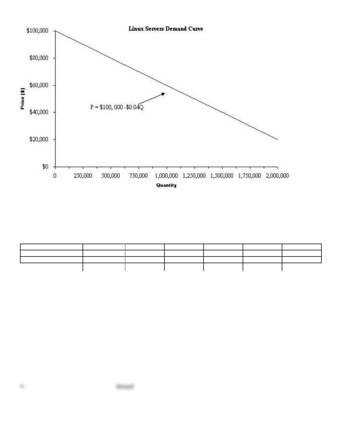
31. Demand Curve Estimation. Linux Servers, Inc., is a leading supplier of high-speed servers with enormous
storage capacity. Average price and annual unit sales data for the VAX-7500 high-speed machine are as
follows:
2001
2002
2003
2004
2005
Price($)
$90,000
$80,000
$60,000
$50,000
$30,000
Units sold
250,000
500,000
1,000,000
1,250,000
1,750,000
A.
Complete the following table, and use these data to derive intercept and slope coefficients for the linear demand curve.
Year
Price
Quantity
¶ Price
¶ Quantity
Slope
= ¶P/ ¶Q
2004
$90,000
250,000
—
—
—
2005
80,000
500,000
2006
60,000
1,000,000
2007
50,000
1,250,000
2008
30,000
1,750,000
B.
Assuming that demand conditions are held constant, use the preceding data to plot a linear demand curve.
A.
True. If r = 1, there is a perfect direct linear relation between the dependent Y variable and the independent X variable.
C.
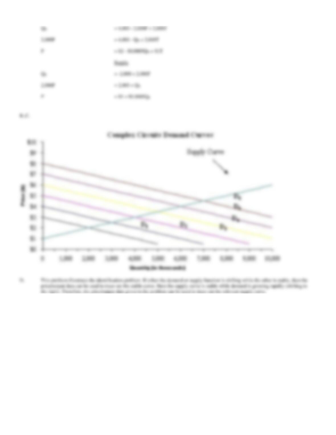
32. The Identification Problem. Business is booming for Complex Controls, Inc., a leading supplier of
analog/digital circuits and systems used for measurement and control. The average price received by CCI for
the XKE device, and the number sold (output) over the past six quarters are as follows:
Q-1
Q-2
Q-3
Q-4
Q-5
Q-6
Price($)
$2.00
$2.50
$3.00
$3.50
$4.00
$4.50
Output(000)
2,000
3,000
4,000
5,000
6,000
7,000
Quarterly demand and supply curves for CCI services are:
QD
= 4,000 – 2,000P + 2,000T
(Demand)
QS
= -2,000 + 2,000P
(Supply)
where Q is output (000), P is price, T is a trend factor, and T = 1 during Q–1 and increases by one unit per quarter.
A.
Express each demand and supply curve in terms of price as a function of output.
B.
Plot the quarterly demand curves for the last six quarterly periods. (Hint: Let T = 1 to find the Y-intercept for Q-1, T = 2 for Q-2, and so
on.)
C.
Plot the CCI supply curve on the same graph.
D.
What is this problem’s relation to the identification problem?
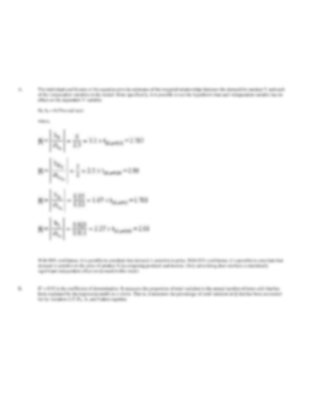
33. R2 and t statistics. Boris Yeltsin Products, Inc., has hired you to analyze demand in 30 regional markets for
Product Y, a new vodka beverage. A statistical analysis of demand in these markets shows (standard errors in
parentheses):
QY
= 500 – 8P + 5PX + 0.05A + 0.025I
(350) (2.5) (2) (0.03) (0.011)
R2
= 93%
QD
= 4,000 – 2,000P + 2,000T
2,000P
= 4,000 – QD + 2,000T
P
= $2 – $0.0005QD + $1T
Supply
QS
2,000P
= 2,000 + QS
P
= $1 + $0.0005QS
B.,C.
Standard Error of the Estimate = 20
Here, QY is market demand for Product Y, P is the price of Y in dollars, A is dollars of advertising expenditures, PX is the average price in dollars of
another (unidentified) product, and I is dollars of household income. In a typical market, the price of Y is $500, PX is $600, advertising expenditures
are $10,000, and average per capita income is $40,000.
A.
Does each independent X variable have a significant effect on the dependent Y variable?
B.
What percentage of demand variation is explained by this model?
where,
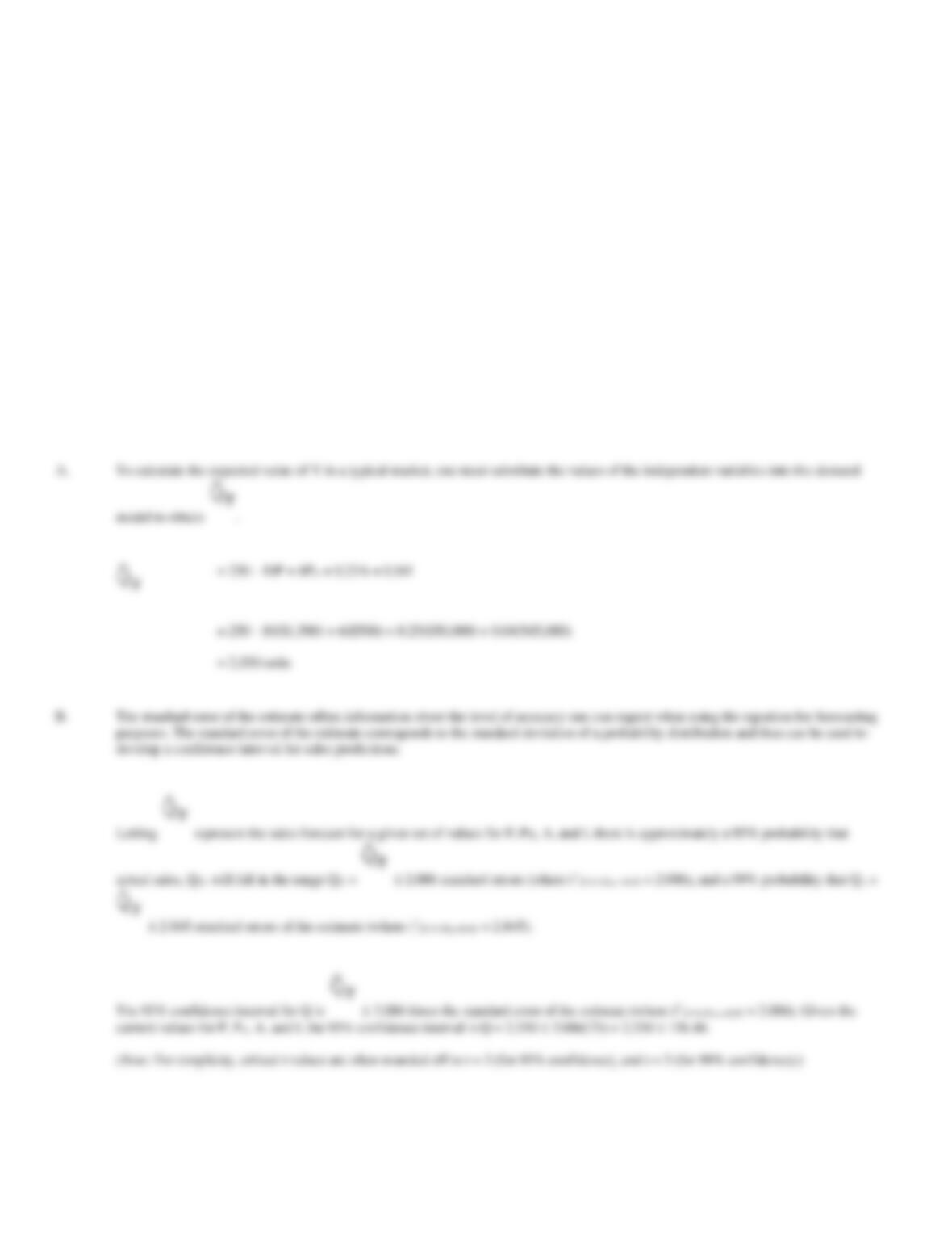
34. Expected Demand Estimation. Snack Foods International, Ltd. has hired you to analyze demand in 25
regional markets for a new Product Y, called Angelica Pickles. A statistical analysis of demand in these markets
shows (standard errors in parentheses):
QY
= 250 – 10P + 6PX + 0.25A + 0.04I
(100) (3) (2) (0.1) (0.15)
R2
= 90%
Standard Error of the Estimate = 75
Here, QY is market demand for Product Y, P is the price of Y in dollars, A is dollars of advertising expenditures, PX is the average price in dollars of
another (unidentified) product, and I is dollars of household income. In a typical market, the price of Y is $1,500, PX is $500, advertising
expenditures are $50,000, and disposable income per household is $45,000.
A.
Calculate the expected level of demand in a typical market.
B.
Indicate the range within which actual demand is expected to fall with 95% confidence.
model to obtain .
= 250 – 10($1,500) + 6($500) + 0.25($50,000) + 0.04($45,000)
= 2,550 units
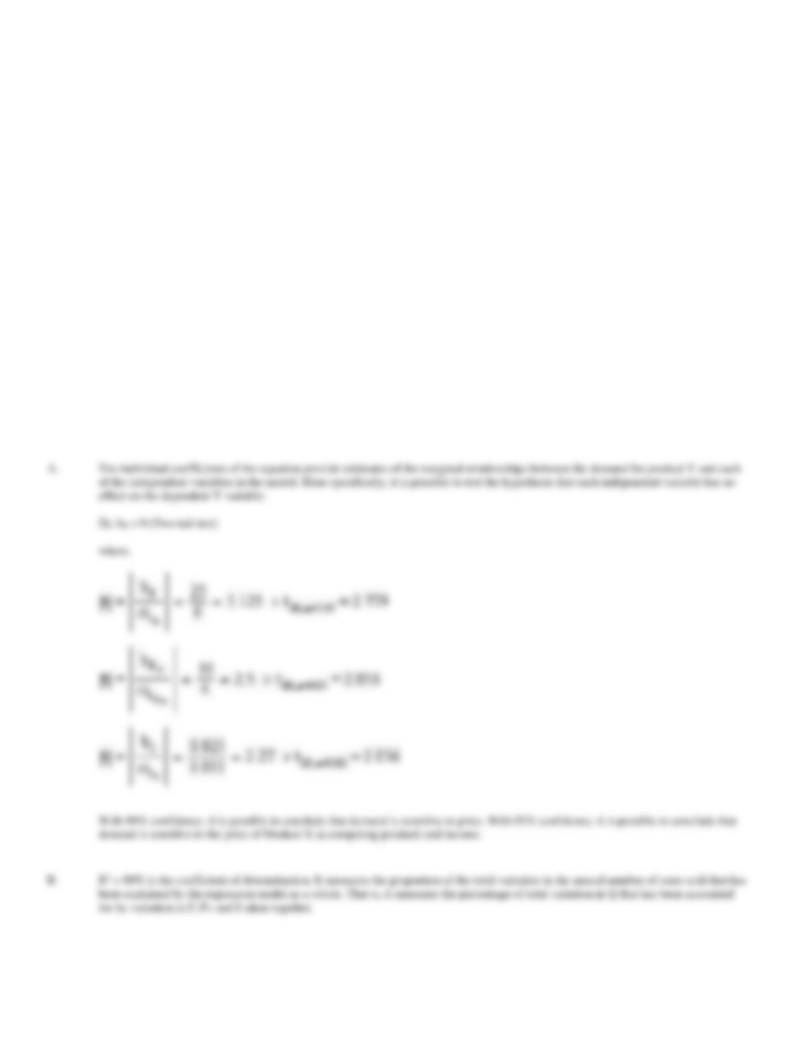
35. Regression Statistics. June Ward, controller for NAFTA, Inc., has asked you to analyze demand in 30
regional markets for Beaver’s Cleavers, a new brush cutting device, dubbed Product Y. A statistical analysis of
demand in these markets shows (standard errors in parentheses):
QY
= 2,000 – 25P + 10PX + 0.025I
(1,500) (8) (4) (0.011)
R2
= 80%
F
= 34.7
Standard Error of the Estimate = 40
Here, QY is market demand for Product Y, P is the price of Y in dollars, A is dollars of advertising expenditures, PX is the average price in dollars of
another (unidentified) product, and I is dollars of household income. In a typical market, the price of Y is $100, PX is $50, and disposable income per
family averages $80,000.
A.
Does each independent X variable have a significant effect on the dependent Y variable?
B.
What percentage of demand variation is explained by this model?
C.
Does this model explain a significant share of demand variation?
D.
Calculate the expected level of demand in a typical market. Also indicate the range within which actual demand is expected to fall with
95% confidence.
H0: bk = 0 (Two-tail test)
where,
36. Price Elasticity Estimation. Thomas Magnum, a financial analyst for Detroit Wheels, Inc., has been hired
to analyze demand in 20 regional markets for Product Y, a major item. A statistical analysis of demand in these
markets shows (standard errors in parentheses):
QY
= 26,950 – 420P + 250PX + 0.05A + 0.01I
(11,000) (160) (180) (0.4) (0.05)
R2
= 0.95
Standard Error of the Estimate = 10
Here, QY is market demand for Product Y, P is the price of Y in dollars, A is dollars of advertising expenditures, PX is the average price in dollars of
another (unidentified) product, and I is dollars of household income. In a typical market, the price of Y is $100, PX is $75, advertising expenditures
are $50,000, and average family income is $80,000.
A.
Use the estimated demand function to calculate the expected value of QY in a typical market.
B.
Calculate the 99% confidence interval within which you would expect to find actual values of sales.
C.
Calculate the point price elasticity of demand.
D.
Would a reduction in price result in an increase in total revenues? Why? or Why not?
model to obtain .
= 26,950 – 420($100) + 250($75) + 0.05($50,000) + 0.01($80,000)
= 7,000 units
As in part C, = 7,000 units.
Therefore,
D.
A price reduction would increase total revenue since demand is elastic (|eP| > 1).
37. Regression Statistics. Financial Planning Associates, Ltd., has hired you to analyze demand in 30 regional
markets for custom financial plans for high net worth individuals (Product Y). A statistical analysis of demand
in these markets shows (standard errors in parentheses):
QY
= 2,000 – 5P – 2.5PX + 0.0825A + 0.005
(1,000) (1.5) (1.2) (0.05) (0.002)
R2
= 0.96
F
= 23.8
Standard Error of the Estimate = 5
Here, QY is market demand for Product Y, P is the price of Y in dollars, A is dollars of advertising expenditures, PX is the average price in dollars of
another (unidentified) product, and I is dollars of household income. In a typical market, the price of Y is $2,000, PX is $1,000, advertising
expenditures are $120,000, and average family income is $200,000.
A.
Briefly interpret the demand equation and explain the use of the regression statistics provided.
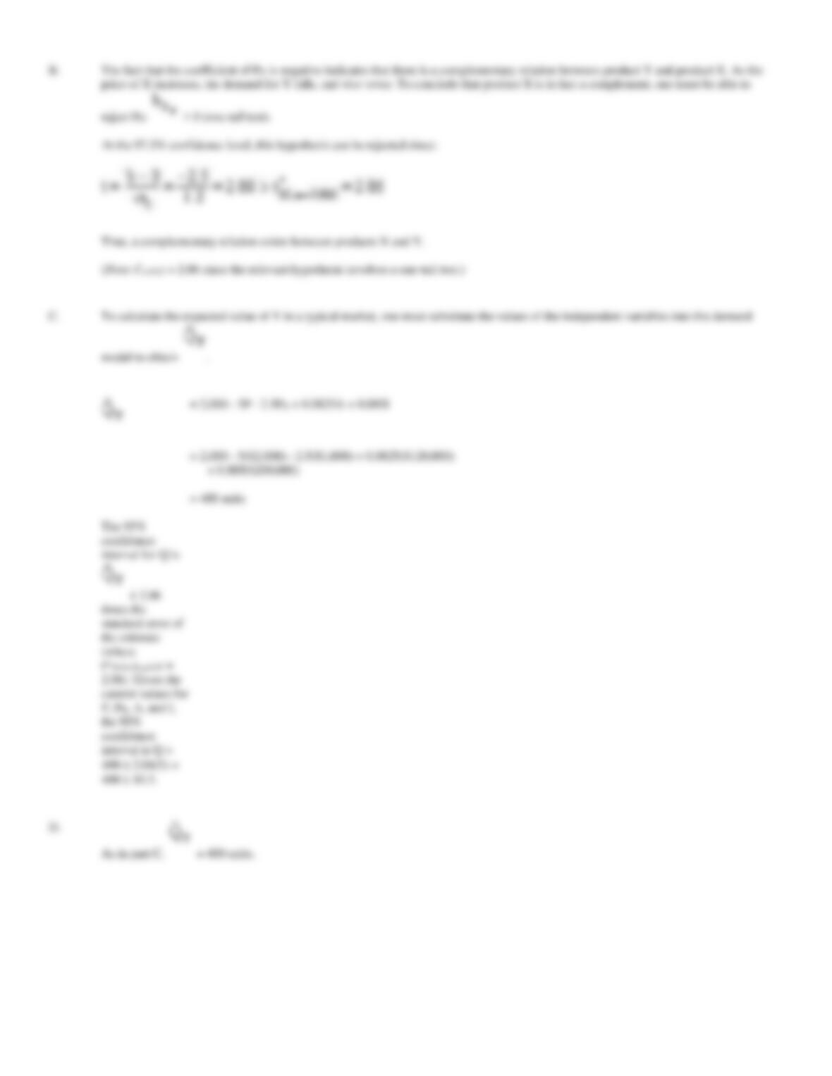
B.
Because of a mix-up in labeling, the PX variable is unidentified. Can you determine at the 95% confidence level whether X is a
complement or a substitute? Why or why not? If so, which is it?
C.
Use the estimated demand function to calculate the expected value of QY in a typical market. Also calculate the 95% confidence interval
within which you would expect to find the actual values of sales.
D.
Calculate the point price elasticity of demand. Would a reduction in price result in an increase in total revenues? Why? or Why not?
advertising, plus 0.005 times household income.
effect on the dependent Y variable:
H0: bk = 0 (Two-tail test)
where,
38. Elasticity Estimation. The Lincoln National Life Insurance Company offers a wide variety of insurance
products, including whole-life and term policies. The company has compiled the following data concerning
policy sales during recent years:
Year
Whole-life
Term
Price*
Quantity
Price*
Quantity
2004
$2.00
240,000
$1.50
100,000
2005
2.00
200,000
1.45
130,000
2006
1.90
230,000
1.45
150,000
2007
1.80
280,000
1.40
200,000
2008
1.80
238,000
1.33
270,000
*Price is quoted in terms of cost per $1,000 of coverage.
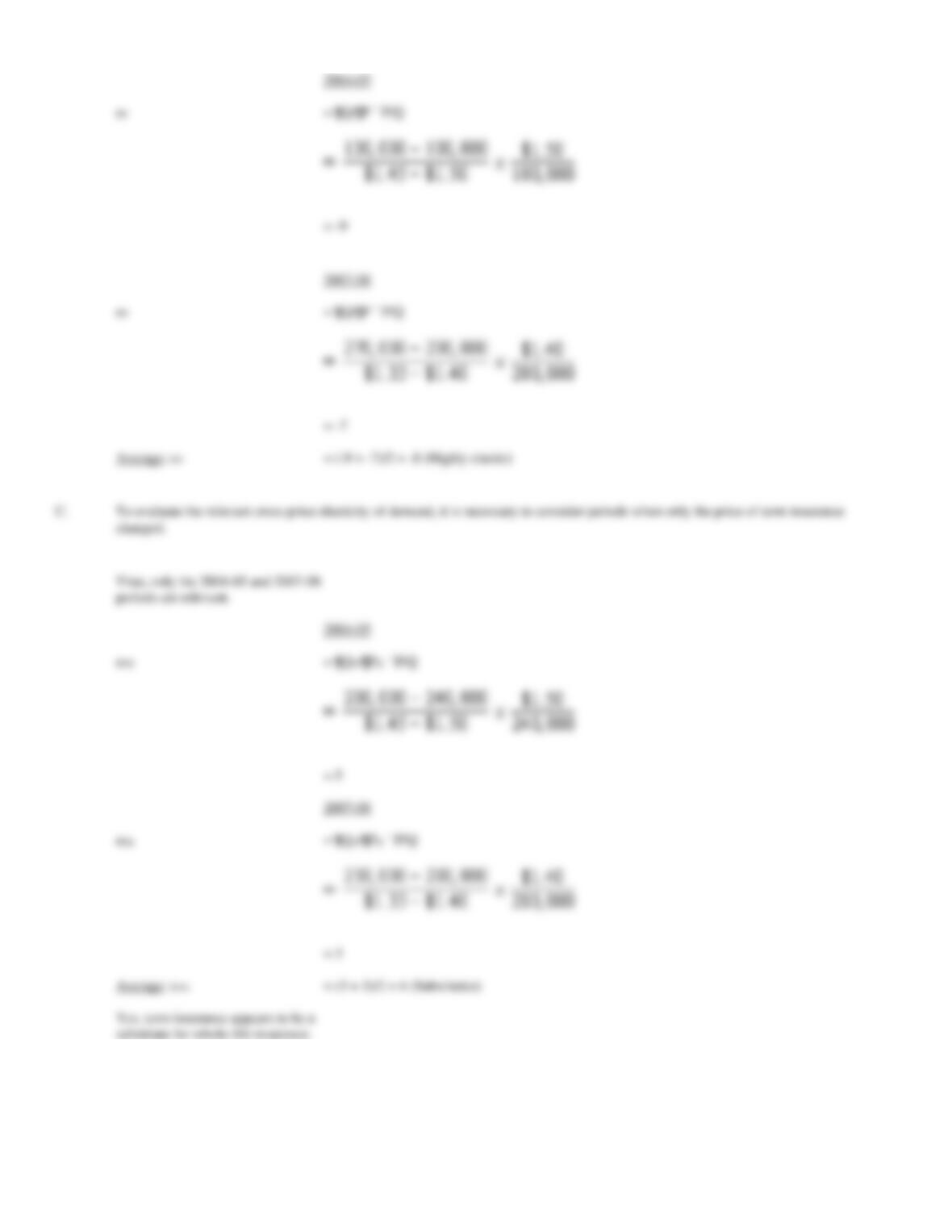
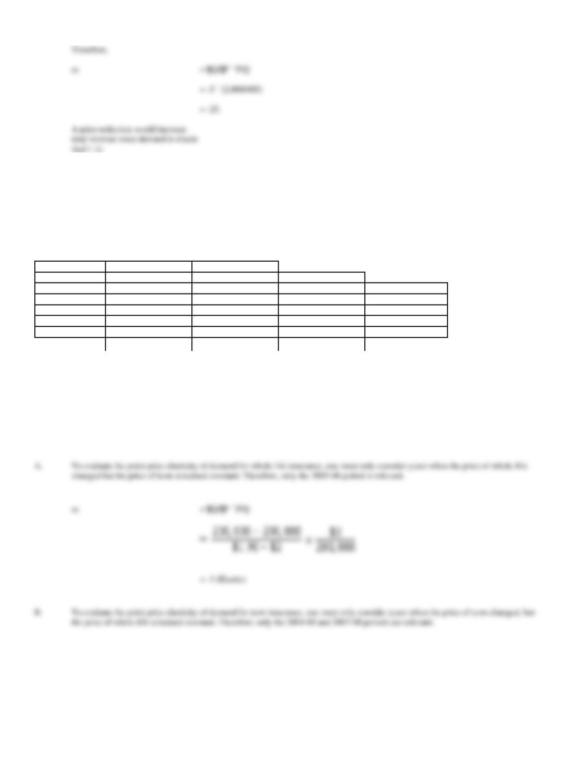
A.
What is the point price elasticity of demand for whole-life insurance?
B.
What is the point price elasticity of demand for term insurance?
C.
Evaluate the percentage change in whole-life demand given a 1% change in the price of term insurance. Is term insurance a substitute
for whole-life?
To evaluate the point price elasticity of demand for whole-life insurance, one must only consider years when the price of whole-life
B.
To evaluate the point price elasticity of demand for term insurance, one must only consider years when the price of term changed, but
the price of whole-life remained constant. Therefore, only the 2004-05 and 2007-08 periods are relevant.
Therefore,