18

19
Copyright © 2015 Pearson Education, Inc.
11) At the Stock and Watson (http://www.pearsonhighered.com/stock_watson) website go to Student
Resources and select the option “Datasets for Replicating Empirical Results.” Then select the “California
Test Score Data Used in Chapters 4–9″ (caschool.xls) and open it in a spreadsheet program such as Excel.
In this exercise you will estimate various statistics of the Linear Regression Model with One Regressor
through construction of various sums and ratio within a spreadsheet program.
Throughout this exercise, let Y correspond to Test Scores (testscore) and X to the Student Teacher
Ratio (str). To generate answers to all exercises here, you will have to create seven columns and the sums
of five of these. They are
(i) Yi, (ii) Xi, (iii) (Yi–
Y
), (iv) (Xi–
X
), (v) (Yi–
Y
)×(Xi–
X
), (vi) (Xi–
X
)2, (vii) (Yi–
Y
)2
Although neither the sum of (iii) or (iv) will be required for further calculations, you may want to
generate these as a check (both have to sum to zero).
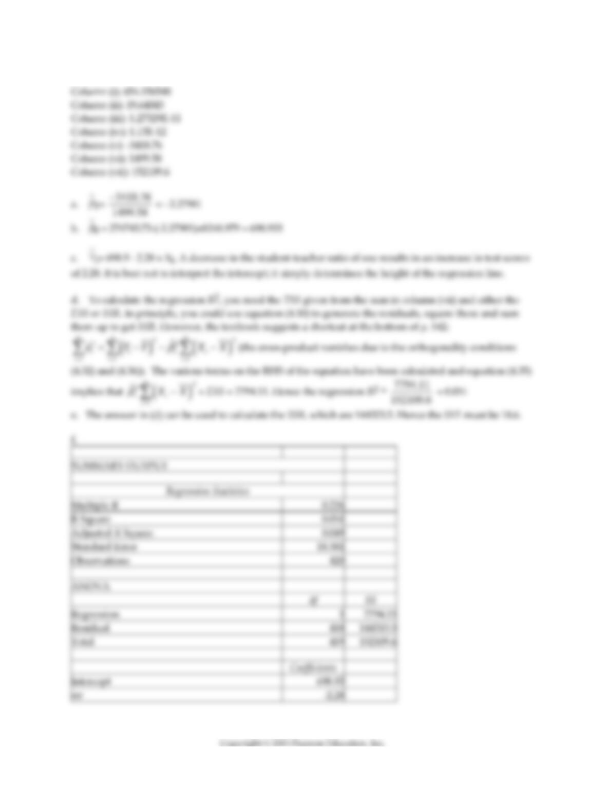
a. Use equation (4.7) and the sums of columns (v) and (vi) to generate the slope of the regression.
b. Use equation (4.8) to generate the intercept.
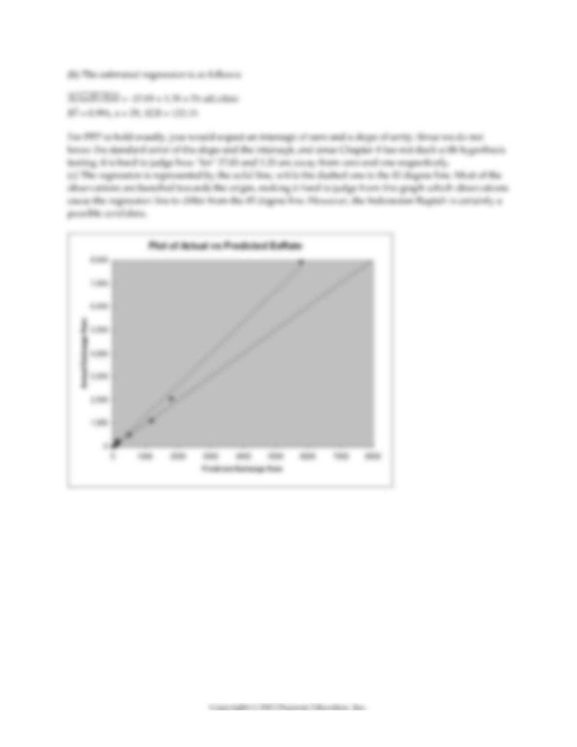
c. Display the regression line (4.9) and interpret the coefficients.
d. Use equation (4.16) and the sum of column (vii) to calculate the regression R2.
e. Use equation (4.19) to calculate the SER.
f. Use the “Regression” function in Excel to verify the results.
20
Answer:
12) You have obtained a sample of 14,925 individuals from the Current Population Survey (CPS) and are
interested in the relationship between average hourly earnings and years of education. The regression
yields the following result:
ˆ
ahe
= –4.58 + 1.71×educ , R2 = 0.182, SER = 9.30
where ahe and educ are measured in dollars and years respectively.
a. Interpret the coefficients and the regression R2.
b. Is the effect of education on earnings large?
c. Why should education matter in the determination of earnings? Do the results suggest that there is a
guarantee for average hourly earnings to rise for everyone as they receive an additional year of
education? Do you think that the relationship between education and average hourly earnings is linear?
d. The average years of education in this sample is 13.5 years. What is mean of average hourly earnings
in the sample?
e. Interpret the measure SER. What is its unit of measurement.
4.3 Mathematical and Graphical Problems
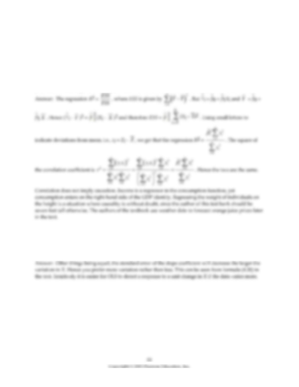
1) Prove that the regression R2 is identical to the square of the correlation coefficient between two
variables Y and X. Regression functions are written in a form that suggests causation running from X to
Y. Given your proof, does a high regression R2 present supportive evidence of a causal relationship? Can
you think of some regression examples where the direction of causality is not clear? Is without a doubt?
2) You have analyzed the relationship between the weight and height of individuals. Although you are
quite confident about the accuracy of your measurements, you feel that some of the observations are
extreme, say, two standard deviations above and below the mean. Your therefore decide to disregard
these individuals. What consequence will this have on the standard deviation of the OLS estimator of the
slope?
3) In order to calculate the regression R2 you need the TSS and either the SSR or the ESS. The TSS is fairly
straightforward to calculate, being just the variation of Y. However, if you had to calculate the SSR or ESS
by hand (or in a spreadsheet), you would need all fitted values from the regression function and their
deviations from the sample mean, or the residuals. Can you think of a quicker way to calculate the ESS
simply using terms you have already used to calculate the slope coefficient?
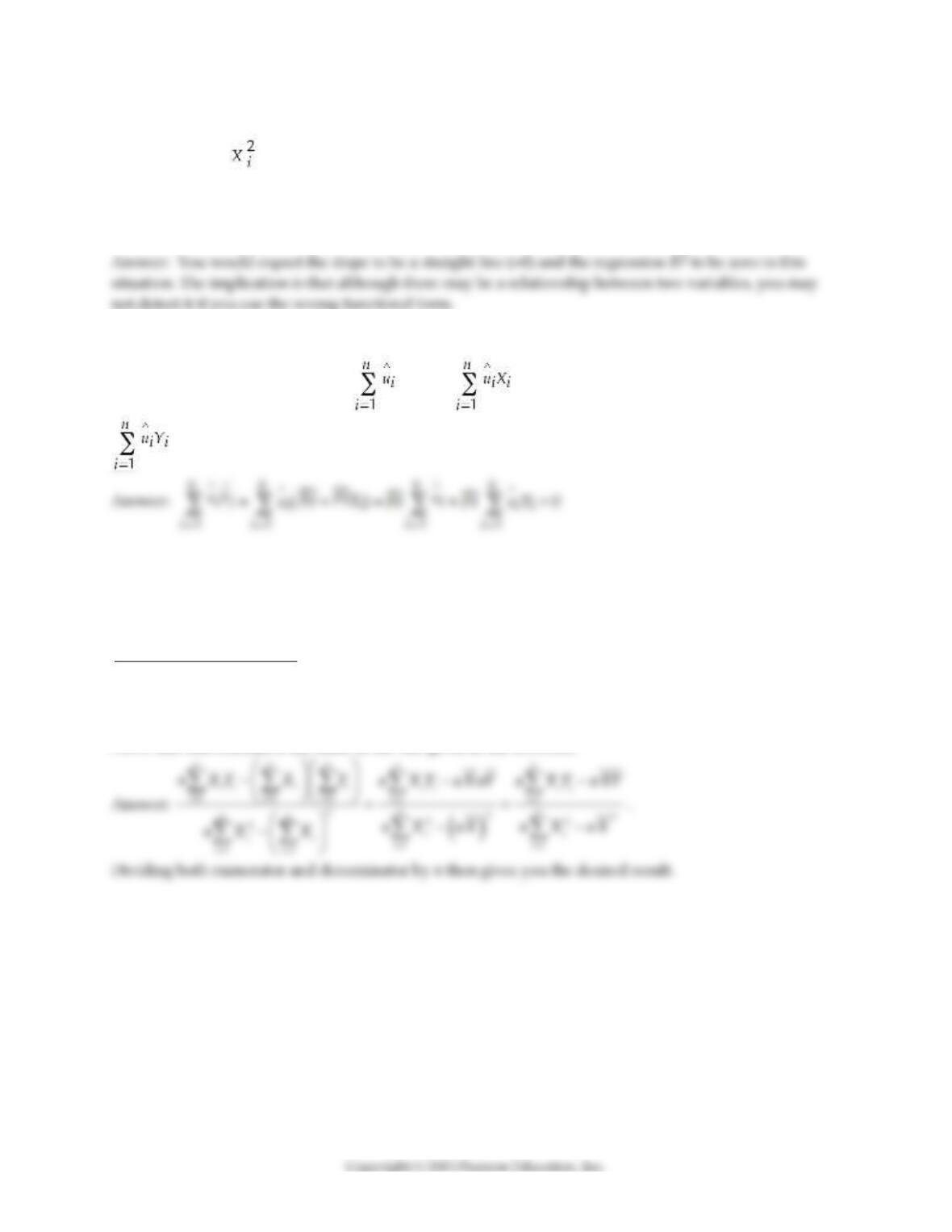
4) (Requires Appendix material) In deriving the OLS estimator, you minimize the sum of squared
residuals with respect to the two parameters 0 and 1. The resulting two equations imply two
restrictions that OLS places on the data, namely that
1
ˆ0
n
i
i
u
=
=
and
1
ˆ0
n
ii
i
uX
=
=
. Show that you get the
same formula for the regression slope and the intercept if you impose these two conditions on the sample
regression function.
1
n
ii
i
uX
=
=
5) (Requires Appendix material) Show that the two alternative formulae for the slope given in your
textbook are identical.
( )( )
( )
11
2
2
2
11
1
1
nn
i i i i
ii
nn
ii
ii
X Y XY X X Y Y
n
X X X X
n
==
==
− − −
=
−−
6) (Requires Calculus) Consider the following model:
Yi = β0 + ui.
Derive the OLS estimator for β0.
n
25
7) (Requires Calculus) Consider the following model:
Yi = β1Xi + ui.
Derive the OLS estimator for β1.
n
8) Show first that the regression R2 is the square of the sample correlation coefficient. Next, show that the
slope of a simple regression of Y on X is only identical to the inverse of the regression slope of X on Y if
the regression R2 equals one.
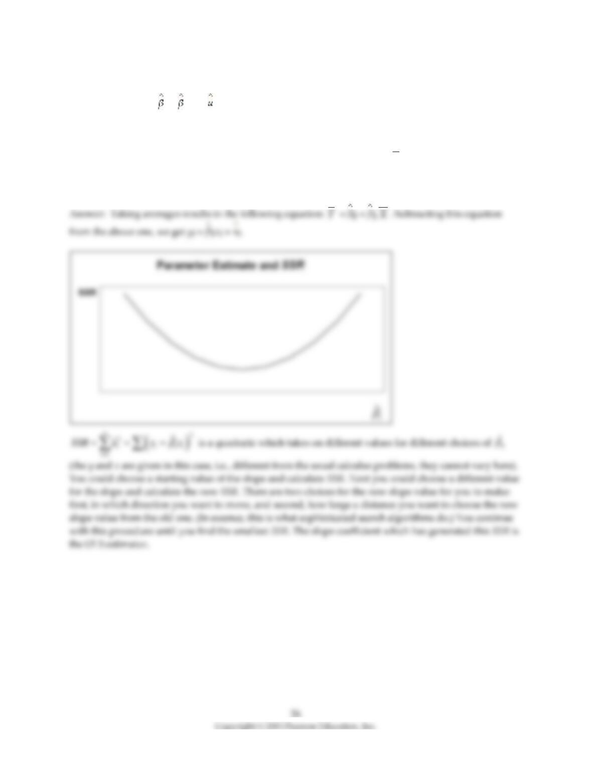
9) Consider the sample regression function
Yi = 0 + 1Xi + i.
First, take averages on both sides of the equation. Second, subtract the resulting equation from the above
equation to write the sample regression function in deviations from means. (For simplicity, you may
want to use small letters to indicate deviations from the mean, i.e., zi = Zi –
Z
.) Finally, illustrate in a
two–dimensional diagram with SSR on the vertical axis and the regression slope on the horizontal axis
how you could find the least squares estimator for the slope by varying its values through trial and error.
10) Given the amount of money and effort that you have spent on your education, you wonder if it was
(is) all worth it. You therefore collect data from the Current Population Survey (CPS) and estimate a
linear relationship between earnings and the years of education of individuals. What would be the effect
on your regression slope and intercept if you measured earnings in thousands of dollars rather than in
dollars? Would the regression R2 be affected? Should statistical inference be dependent on the scale of
variables? Discuss.
11) (Requires Appendix material) Consider the sample regression function
**
01
ˆˆ ˆ
i i i
Y X u
= + +
,
where * indicates that the variable has been standardized. What are the units of measurement for the
dependent and explanatory variable? Why would you want to transform both variables in this way?
Show that the OLS estimator for the intercept equals zero. Next prove that the OLS estimator for the slope
in this case is identical to the formula for the least squares estimator where the variables have not been
standardized, times the ratio of the sample standard deviation of X and Y, i.e.,
11
ˆ
ˆX
Y
S
S
=
.
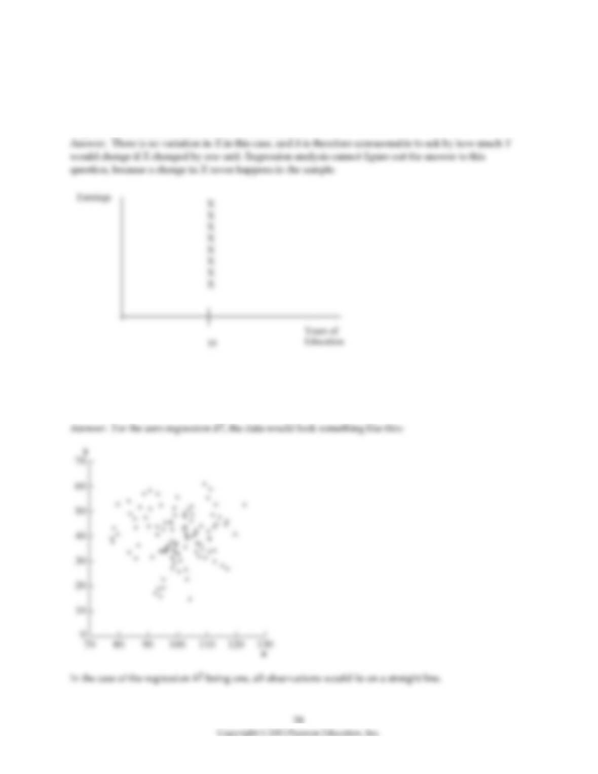
12) The OLS slope estimator is not defined if there is no variation in the data for the explanatory variable.
You are interested in estimating a regression relating earnings to years of schooling. Imagine that you
had collected data on earnings for different individuals, but that all these individuals had completed a
college education (16 years of education). Sketch what the data would look like and explain intuitively
why the OLS coefficient does not exist in this situation.
13) Indicate in a scatterplot what the data for your dependent variable and your explanatory variable
would look like in a regression with an R2 equal to zero. How would this change if the regression R2 was
equal to one?
29
14) Imagine that you had discovered a relationship that would generate a scatterplot very similar to the
relationship Yi = , and that you would try to fit a linear regression through your data points. What do
you expect the slope coefficient to be? What do you think the value of your regression R2 is in this
situation? What are the implications from your answers in terms of fitting a linear regression through a
non–linear relationship?
15) (Requires Appendix material) A necessary and sufficient condition to derive the OLS estimator is that
the following two conditions hold: = 0 and = 0. Show that these conditions imply that
= 0.
16) The help function for a commonly used spreadsheet program gives the following definition for the
regression slope it estimates:
1 1 1
2
2
11
n n n
i i i i
i i i
nn
ii
ii
n X Y X Y
n X X
= = =
==
−
−
Prove that this formula is the same as the one given in the textbook.
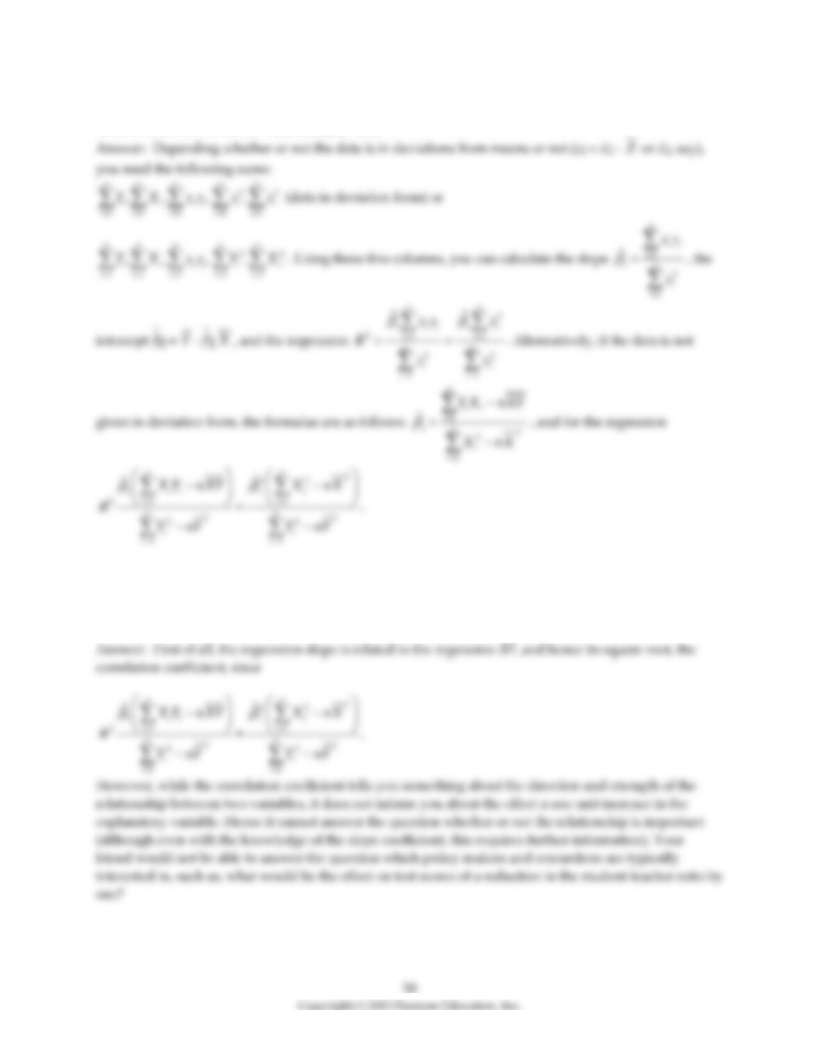
17) In order to calculate the slope, the intercept, and the regression R2 for a simple sample regression
function, list the five sums of data that you need.
18) A peer of yours, who is a major in another social science, says he is not interested in the regression
slope and/or intercept. Instead he only cares about correlations. For example, in the testscore/student–
teacher ratio regression, he claims to get all the information he needs from the negative correlation
coefficient corr(X,Y)=-0.226. What response might you have for your peer?
19) Assume that there is a change in the units of measurement on both Y and X. The new variables are
Y*= aY and X* = bX. What effect will this change have on the regression slope?
20) Assume that there is a change in the units of measurement on X. The new variables X* = bX. Prove
that this change in the units of measurement on the explanatory variable has no effect on the intercept in
the resulting regression.
21) At the Stock and Watson (http://www.pearsonhighered.com/stock_watson) website, go to Student
Resources and select the option “Datasets for Replicating Empirical Results.” Then select the “California
Test Score Data Used in Chapters 4–9″ and read the data either into Excel or STATA (or another statistical
program). First run a regression where the dependent variable is test scores and the independent variable
is the student–teacher ratio. Record the regression R2. Then run a regression where the dependent
variable is the student–teacher ratio and the independent variable is test scores. Record the regression R2
from this regression. How do they compare?
22) At the Stock and Watson (http://www.pearsonhighered.com/stock_watson) website, go to Student
Resources and select the option “Datasets for Replicating Empirical Results.” Then select the “California
Test Score Data Used in Chapters 4–9″ and read the data either into Excel or STATA (or another statistical
program).
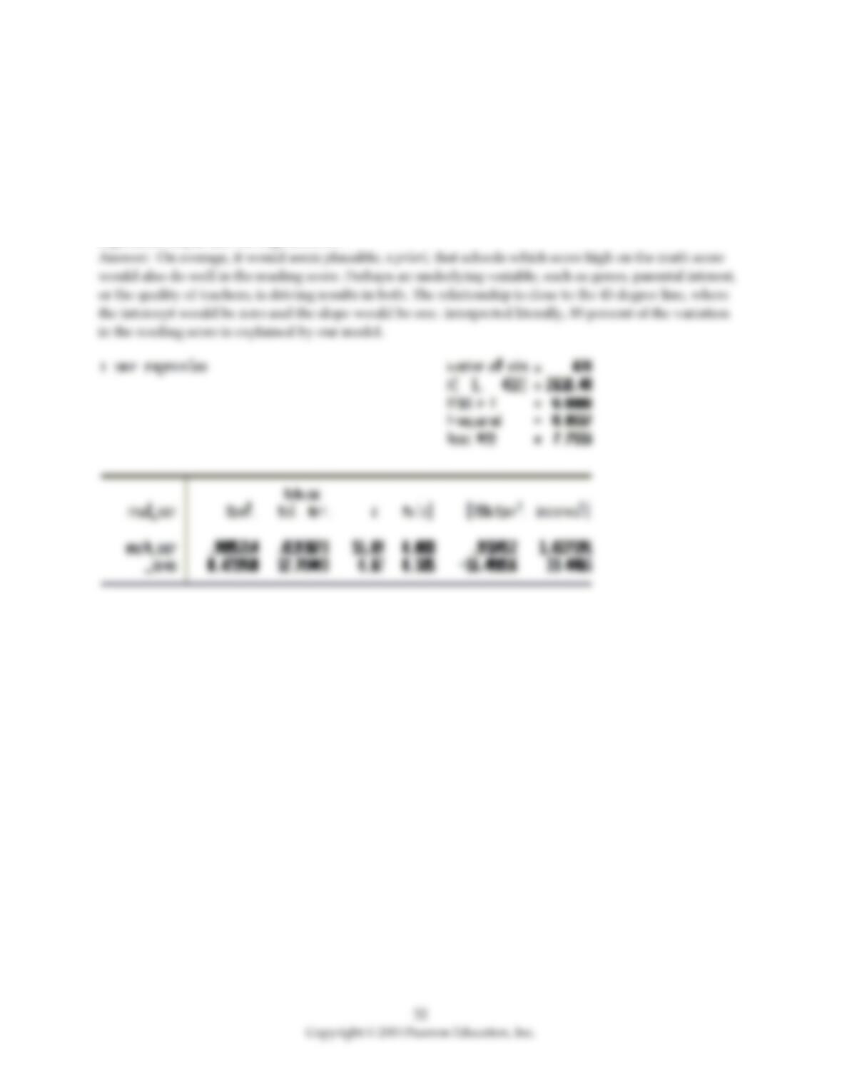
Run a regression of the average reading score (read_scr) on the average math score (math_scr). What
values for the slope and the intercept would you expect? Interpret the coefficients in the resulting
regression output and the regression R2.
23) In a simple regression with an intercept and a single explanatory variable, the variation in Y
( )
2
1
()
n
i
i
TSS Y Y
=
=−
can be decomposed into the explained sums of squares
( )
2
1
ˆ
()
n
i
i
ESS Y Y
=
=−
and the
sum of squared residuals
( )
2
2
11
ˆ
ˆ
()
nn
ii
ii
SSR u Y Y
==
= = −
(see, for example, equation (4.35) in the textbook).
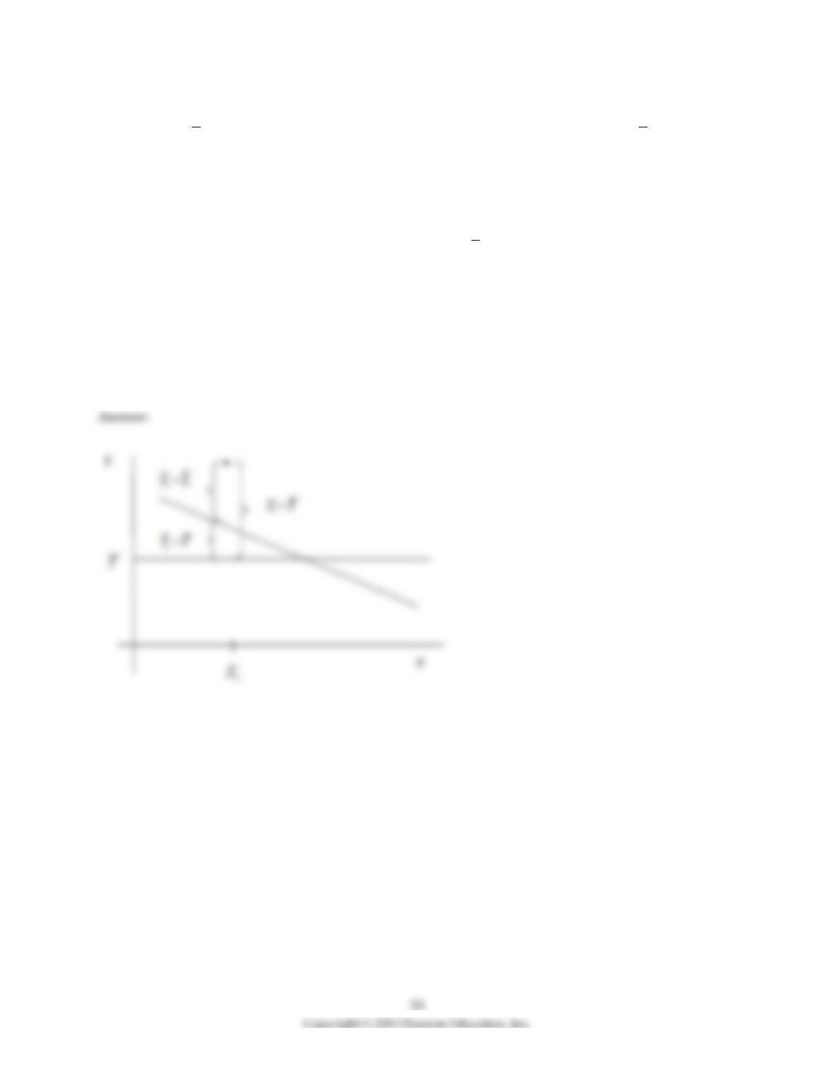
Consider any regression line, positively or negatively sloped in {X,Y} space. Draw a horizontal line
where, hypothetically, you consider the sample mean of Y
( )
Y=
to be. Next add a single actual
observation of Y.
In this graph, indicate where you find the following distances: the
(i) residual
(ii) actual minus the mean of Y
(iii) fitted value minus the mean of Y