
Introduction to Econometrics, 3e (Stock)
Chapter 4 Linear Regression with One Regressor
4.1 Multiple Choice
1) When the estimated slope coefficient in the simple regression model, 1, is zero, then
A) R2 = .
B) 0 < R2 < 1.
C) R2 = 0.
D) R2 > (SSR/TSS).
2) The regression R2 is defined as follows:
A)
ESS
TSS
B)
RSS
TSS
C)
( )( )
( ) ( )
1
22
11
n
ii
i
nn
ii
ii
Y Y X X
Y Y X X
=
==
−−
−−
D)
2
SSR
n−
3) The standard error of the regression (SER) is defined as follows
A)
2
1
1ˆ
2
n
i
i
u
n=
−
B) SSR
C) 1–R2
D)
2
1
1ˆ
1
n
i
i
u
n=
−
4) (Requires Appendix material) Which of the following statements is correct?
A) TSS = ESS + SSR
B) ESS = SSR + TSS
C) ESS > TSS
D) R2 = 1 – (ESS/TSS)

5) Binary variables
A) are generally used to control for outliers in your sample.
B) can take on more than two values.
C) exclude certain individuals from your sample.
D) can take on only two values.
6) The following are all least squares assumptions with the exception of:
A) The conditional distribution of ui given Xi has a mean of zero.
B) The explanatory variable in regression model is normally distributed.
C) (Xi, Yi), i = 1,…, n are independently and identically distributed.
D) Large outliers are unlikely.
7) The reason why estimators have a sampling distribution is that
A) economics is not a precise science.
B) individuals respond differently to incentives.
C) in real life you typically get to sample many times.
D) the values of the explanatory variable and the error term differ across samples.
8) In the simple linear regression model, the regression slope
A) indicates by how many percent Y increases, given a one percent increase in X.
B) when multiplied with the explanatory variable will give you the predicted Y.
C) indicates by how many units Y increases, given a one unit increase in X.
D) represents the elasticity of Y on X.
9) The OLS estimator is derived by
A) connecting the Yi corresponding to the lowest Xi observation with the Yi corresponding to the highest
Xi observation.
B) making sure that the standard error of the regression equals the standard error of the slope estimator.
C) minimizing the sum of absolute residuals.
D) minimizing the sum of squared residuals.
10) Interpreting the intercept in a sample regression function is
A) not reasonable because you never observe values of the explanatory variables around the origin.
B) reasonable because under certain conditions the estimator is BLUE.
C) reasonable if your sample contains values of Xi around the origin.
D) not reasonable because economists are interested in the effect of a change in X on the change in Y.

11) The variance of Yi is given by
A) + var(Xi) + var(ui).
B) the variance of ui.
C)
var(Xi) + var(ui).
D) the variance of the residuals.
12) (Requires Appendix) The sample average of the OLS residuals is
A) some positive number since OLS uses squares.
B) zero.
C) unobservable since the population regression function is unknown.
D) dependent on whether the explanatory variable is mostly positive or negative.
13) The OLS residuals, i, are defined as follows:
A) i – 0 – 1Xi
B) Yi – β0 – β1Xi
C) Yi – i
D) (Yi – )2
14) The slope estimator, β1, has a smaller standard error, other things equal, if
A) there is more variation in the explanatory variable, X.
B) there is a large variance of the error term, u.
C) the sample size is smaller.
D) the intercept, β0, is small.
15) The regression R2 is a measure of
A) whether or not X causes Y.
B) the goodness of fit of your regression line.
C) whether or not ESS > TSS.
D) the square of the determinant of R.
16) (Requires Appendix) The sample regression line estimated by OLS
A) will always have a slope smaller than the intercept.
B) is exactly the same as the population regression line.
C) cannot have a slope of zero.
D) will always run through the point ( , ).

17) The OLS residuals
A) can be calculated using the errors from the regression function.
B) can be calculated by subtracting the fitted values from the actual values.
C) are unknown since we do not know the population regression function.
D) should not be used in practice since they indicate that your regression does not run through all your
observations.
18) The normal approximation to the sampling distribution of 1 is powerful because
A) many explanatory variables in real life are normally distributed.
B) it allows econometricians to develop methods for statistical inference.
C) many other distributions are not symmetric.
D) is implies that OLS is the BLUE estimator for β1.
19) If the three least squares assumptions hold, then the large sample normal distribution of 1 is
A)
( )
2
var )
1
0,
var
i X i
i
Xu
NnX
−
.
B)
( )
( )
2
12
var ]
1
,
var
i
i
u
NnX
.
C)
( )
2
12
1
(, u
n
i
i
N
XX
=
−
.
D)
( )
( )
12
var ]
1
,
var
i
i
u
NnX
.
20) In the simple linear regression model Yi = β0 + β1Xi + ui,
A) the intercept is typically small and unimportant.
B) β0 + β1Xi represents the population regression function.
C) the absolute value of the slope is typically between 0 and 1.
D) β0 + β1Xi represents the sample regression function.
21) To obtain the slope estimator using the least squares principle, you divide the
A) sample variance of X by the sample variance of Y.
B) sample covariance of X and Y by the sample variance of Y.
C) sample covariance of X and Y by the sample variance of X.
D) sample variance of X by the sample covariance of X and Y.

22) To decide whether or not the slope coefficient is large or small,
A) you should analyze the economic importance of a given increase in X.
B) the slope coefficient must be larger than one.
C) the slope coefficient must be statistically significant.
D) you should change the scale of the X variable if the coefficient appears to be too small.
23) E(uiXi) = 0 says that
A) dividing the error by the explanatory variable results in a zero (on average).
B) the sample regression function residuals are unrelated to the explanatory variable.
C) the sample mean of the Xs is much larger than the sample mean of the errors.
D) the conditional distribution of the error given the explanatory variable has a zero mean.
24) In the linear regression model, Yi = β0 + β1Xi + ui, β0 + β1Xi is referred to as
A) the population regression function.
B) the sample regression function.
C) exogenous variation.
D) the right–hand variable or regressor.
25) Multiplying the dependent variable by 100 and the explanatory variable by 100,000 leaves the
A) OLS estimate of the slope the same.
B) OLS estimate of the intercept the same.
C) regression R2 the same.
D) variance of the OLS estimators the same.
26) Assume that you have collected a sample of observations from over 100 households and their
consumption and income patterns. Using these observations, you estimate the following regression Ci =
β0+β1Yi+ ui where C is consumption and Y is disposable income. The estimate of β1 will tell you
A)
Income
Consumption
B) The amount you need to consume to survive
C)
Income
Consumption
D)
Consumption
Income

27) In which of the following relationships does the intercept have a real–world interpretation?
A) the relationship between the change in the unemployment rate and the growth rate of real GDP
(“Okun’s Law”)
B) the demand for coffee and its price
C) test scores and class–size
D) weight and height of individuals
28) The OLS residuals, i, are sample counterparts of the population
A) regression function slope
B) errors
C) regression function’s predicted values
D) regression function intercept
29) Changing the units of measurement, e.g. measuring testscores in 100s, will do all of the following
EXCEPT for changing the
A) residuals
B) numerical value of the slope estimate
C) interpretation of the effect that a change in X has on the change in Y
D) numerical value of the intercept
30) To decide whether the slope coefficient indicates a “large” effect of X on Y, you look at the
A) size of the slope coefficient
B) regression R2
C) economic importance implied by the slope coefficient
D) value of the intercept
4.2 Essays and Longer Questions
1) Sir Francis Galton, a cousin of James Darwin, examined the relationship between the height of children
and their parents towards the end of the 19th century. It is from this study that the name “regression”
originated. You decide to update his findings by collecting data from 110 college students, and estimate
the following relationship:
= 19.6 + 0.73 × Midparh, R2 = 0.45, SER = 2.0
where Studenth is the height of students in inches, and Midparh is the average of the parental heights.
(Following Galton’s methodology, both variables were adjusted so that the average female height was
equal to the average male height.)
(a) Interpret the estimated coefficients.
(b) What is the meaning of the regression R2?
(c) What is the prediction for the height of a child whose parents have an average height of 70.06 inches?
(d) What is the interpretation of the SER here?
(e) Given the positive intercept and the fact that the slope lies between zero and one, what can you say
about the height of students who have quite tall parents? Those who have quite short parents?
(f) Galton was concerned about the height of the English aristocracy and referred to the above result as
“regression towards mediocrity.” Can you figure out what his concern was? Why do you think that we
refer to this result today as “Galton’s Fallacy”?
2) (Requires Appendix material) At a recent county fair, you observed that at one stand people’s weight
was forecasted, and were surprised by the accuracy (within a range). Thinking about how the person
could have predicted your weight fairly accurately (despite the fact that she did not know about your
“heavy bones”), you think about how this could have been accomplished. You remember that medical
charts for children contain 5%, 25%, 50%, 75% and 95% lines for a weight/height relationship and decide
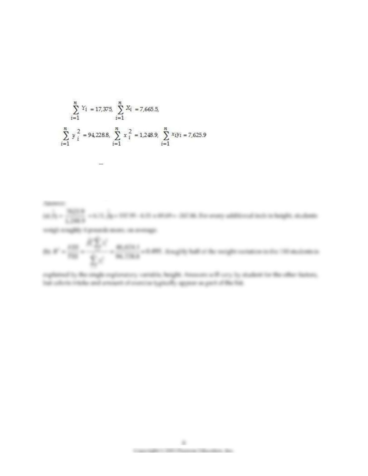
to conduct an experiment with 110 of your peers. You collect the data and calculate the following sums:
where the height is measured in inches and weight in pounds. (Small letters refer to deviations from
means as in zi = Zi –
Z
)
(a) Calculate the slope and intercept of the regression and interpret these.
(b) Find the regression R2 and explain its meaning. What other factors can you think of that might have
an influence on the weight of an individual?
3) You have obtained a sub–sample of 1744 individuals from the Current Population Survey (CPS) and
are interested in the relationship between weekly earnings and age. The regression, using
heteroskedasticity–robust standard errors, yielded the following result:
= 239.16 + 5.20 × Age, R2 = 0.05, SER = 287.21.,
where Earn and Age are measured in dollars and years respectively.
(a) Interpret the results.
(b) Is the effect of age on earnings large?
(c) Why should age matter in the determination of earnings? Do the results suggest that there is a
guarantee for earnings to rise for everyone as they become older? Do you think that the relationship
between age and earnings is linear?
(d) The average age in this sample is 37.5 years. What is annual income in the sample?
(e) Interpret the measures of fit.

10
4) The baseball team nearest to your home town is, once again, not doing well. Given that your
knowledge of what it takes to win in baseball is vastly superior to that of management, you want to find
out what it takes to win in Major League Baseball (MLB). You therefore collect the winning percentage of
all 30 baseball teams in MLB for 1999 and regress the winning percentage on what you consider the
primary determinant for wins, which is quality pitching (team earned run average). You find the
following information on team performance:
Summary of the Distribution of Winning Percentage and
Team Earned Run Average for MLB in 1999
Average
Standard
deviation
Percentile
10%
25%
40%
50%
(median)
60%
75%
90%
Team
ERA
4.71
0.53
3.84
4.35
4.72
4.78
4.91
5.06
5.25
Winning
Percentage
0.50
0.08
0.40
0.43
0.46
0.48
0.49
0.59
0.60
(a) What is your expected sign for the regression slope? Will it make sense to interpret the intercept? If
not, should you omit it from your regression and force the regression line through the origin?
(b) OLS estimation of the relationship between the winning percentage and the team ERA yield the
following:
= 0.9 – 0.10 × teamera , R2=0.49, SER = 0.06,
where winpct is measured as wins divided by games played, so for example a team that won half of its
games would have Winpct = 0.50. Interpret your regression results.
(c) It is typically sufficient to win 90 games to be in the playoffs and/or to win a division. Winning over
100 games a season is exceptional: the Atlanta Braves had the most wins in 1999 with 103. Teams play a
total of 162 games a year. Given this information, do you consider the slope coefficient to be large or
small?
(d) What would be the effect on the slope, the intercept, and the regression R2 if you measured Winpct in
percentage points, i.e., as (Wins/Games) × 100?
(e) Are you impressed with the size of the regression R2? Given that there is 51% of unexplained variation
in the winning percentage, what might some of these factors be?
5) You have learned in one of your economics courses that one of the determinants of per capita income
(the “Wealth of Nations”) is the population growth rate. Furthermore you also found out that the Penn
World Tables contain income and population data for 104 countries of the world. To test this theory, you
regress the GDP per worker (relative to the United States) in 1990 (RelPersInc) on the difference between
the average population growth rate of that country (n) to the U.S. average population growth rate (nus )
for the years 1980 to 1990. This results in the following regression output:
= 0.518 – 18.831 × 18.831 × (n – nus), R2 = 0.522, SER = 0.197
(a) Interpret the results carefully. Is this relationship economically important?
(b) What would happen to the slope, intercept, and regression R2 if you ran another regression where the
above explanatory variable was replaced by n only, i.e., the average population growth rate of the
country? (The population growth rate of the United States from 1980 to 1990 was 0.009.) Should this have
any effect on the t–statistic of the slope?
(c) 31 of the 104 countries have a dependent variable of less than 0.10. Does it therefore make sense to
interpret the intercept?
6) The neoclassical growth model predicts that for identical savings rates and population growth rates,
countries should converge to the per capita income level. This is referred to as the convergence
hypothesis. One way to test for the presence of convergence is to compare the growth rates over time to
the initial starting level.
(a) If you regressed the average growth rate over a time period (1960–1990) on the initial level of per
capita income, what would the sign of the slope have to be to indicate this type of convergence? Explain.
Would this result confirm or reject the prediction of the neoclassical growth model?
(b) The results of the regression for 104 countries were as follows:
= 0.019 – 0.0006 × RelProd60 , R2 = 0.00007, SER = 0.016,
where g6090 is the average annual growth rate of GDP per worker for the 1960–1990 sample period, and
RelProd60 is GDP per worker relative to the United States in 1960.
Interpret the results. Is there any evidence of unconditional convergence between the countries of the
world? Is this result surprising? What other concept could you think about to test for convergence
between countries?
(c) You decide to restrict yourself to the 24 OECD countries in the sample. This changes your regression
output as follows:
= 0.048 – 0.0404 RelProd60 , R2 = 0.82 , SER = 0.0046
How does this result affect your conclusions from above?
14
7) In 2001, the Arizona Diamondbacks defeated the New York Yankees in the Baseball World Series in 7
games. Some players, such as Bautista and Finley for the Diamondbacks, had a substantially higher
batting average during the World Series than during the regular season. Others, such as Brosius and Jeter
for the Yankees, did substantially poorer. You set out to investigate whether or not the regular season
batting average is a good indicator for the World Series batting average. The results for 11 players who
had the most at bats for the two teams are:
= –0.347 + 2.290 AZSeasavg , R2=0.11, SER = 0.145,
= 0.134 + 0.136 NYSeasavg , R2=0.001, SER = 0.092,
where Wsavg and Seasavg indicate the batting average during the World Series and the regular season
respectively.
(a) Focusing on the coefficients first, what is your interpretation?
(b) What can you say about the explanatory power of your equation? What do you conclude from this?
8) For the simple regression model of Chapter 4, you have been given the following data:
420
1
i
i
Y
=
= 274, 745.75;
420
1
i
i
X
=
= 8,248.979;
420
1
ii
i
XY
=
= 5,392, 705;
420
2
1
i
i
X
=
= 163,513.03;
420
2
1
i
i
Y
=
= 179,878, 841.13
(a) Calculate the regression slope and the intercept.
(b) Calculate the regression R2
9) Your textbook presented you with the following regression output:
= 698.9 – 2.28 × STR
n = 420, R2 = 0.051, SER = 18.6
(a) How would the slope coefficient change, if you decided one day to measure testscores in 100s, i.e., a
test score of 650 became 6.5? Would this have an effect on your interpretation?
(b) Do you think the regression R2 will change? Why or why not?
(c) Although Chapter 4 in your textbook did not deal with hypothesis testing, it presented you with the
large sample distribution for the slope and the intercept estimator. Given the change in the units of
measurement in (a), do you think that the variance of the slope estimator will change numerically? Why
or why not?

16
10) The news–magazine The Economist regularly publishes data on the so called Big Mac index and
exchange rates between countries. The data for 30 countries from the April 29, 2000 issue is listed below:
Price of Actual Exchange Rate
Country Currency Big Mac per U.S. dollar
Indonesia Rupiah 14,500 7,945
Italy Lira 4,500 2,088
South Korea Won 3,000 1,108
Chile Peso 1,260 514
Spain Peseta 375 179
Hungary Forint 339 279
Japan Yen 294 106
Taiwan Dollar 70 30.6
Thailand Baht 55 38.0
Czech Rep. Crown 54.37 39.1
Russia Ruble 39.50 28.5
Denmark Crown 24.75 8.04
Sweden Crown 24.0 8.84
Mexico Peso 20.9 9.41
France Franc 18.5 .07
Israel Shekel 14.5 4.05
China Yuan 9.90 8.28
South Africa Rand 9.0 6.72
Switzerland Franc 5.90 1.70
Poland Zloty 5.50 4.30
Germany Mark 4.99 2.11
Malaysia Dollar 4.52 3.80
New Zealand Dollar 3.40 2.01
Singapore Dollar 3.20 1.70
Brazil Real 2.95 1.79
Canada Dollar 2.85 1.47
Australia Dollar 2.59 1.68
Argentina Peso 2.50 1.00
Britain Pound 1.90 0.63
United States Dollar 2.51
The concept of purchasing power parity or PPP (“the idea that similar foreign and domestic goods …
should have the same price in terms of the same currency,” Abel, A. and B. Bernanke, Macroeconomics, 4th
edition, Boston: Addison Wesley, 476) suggests that the ratio of the Big Mac priced in the local currency
to the U.S. dollar price should equal the exchange rate between the two countries.
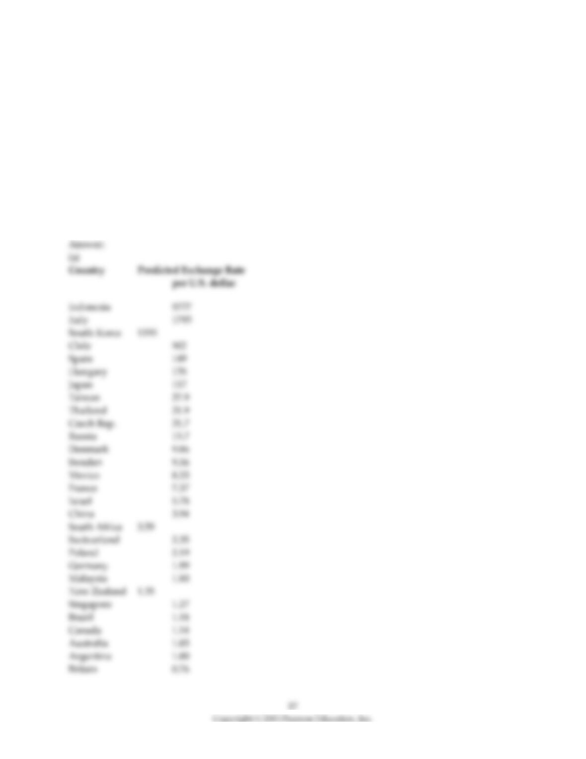
(a) Enter the data into your regression analysis program (EViews, Stata, Excel, SAS, etc.). Calculate the
predicted exchange rate per U.S. dollar by dividing the price of a Big Mac in local currency by the U.S.
price of a Big Mac ($2.51).
(b) Run a regression of the actual exchange rate on the predicted exchange rate. If purchasing power
parity held, what would you expect the slope and the intercept of the regression to be? Is the value of the
slope and the intercept “far” from the values you would expect to hold under PPP?
(c) Plot the actual exchange rate against the predicted exchange rate. Include the 45 degree line in your
graph. Which observations might cause the slope and the intercept to differ from zero and one?