Introduction to Econometrics, 3e (Stock)
Chapter 3 Review of Statistics
3.1 Multiple Choice
1) An estimator is
A) an estimate.
B) a formula that gives an efficient guess of the true population value.
C) a random variable.
D) a nonrandom number.
2) An estimate is
A) efficient if it has the smallest variance possible.
B) a nonrandom number.
C) unbiased if its expected value equals the population value.
D) another word for estimator.
3) An estimator
ˆY
of the population value
Y
is unbiased if
A)
ˆY
=
Y
.
B)
Y
has the smallest variance of all estimators.
C)
Y
p
Y
⎯→⎯
.
D) E(
ˆY
) =
Y
.
4) An estimator
ˆY
of the population value
Y
is consistent if
A)
ˆY
.
B) its mean square error is the smallest possible.
C) Y is normally distributed.
D)
0⎯→⎯p
Y
.
5) An estimator
ˆY
of the population value
Y
is more efficient when compared to another estimator
Y
,
if
A) E(
ˆY
) > E(
Y
).
B) it has a smaller variance.
C) its c.d.f. is flatter than that of the other estimator.
D) both estimators are unbiased, and var(
ˆY
) < var(
Y
).
6) With i.i.d. sampling each of the following is true except
A) E
()Y
=
Y
.
B) var
()Y
=
2
Y
/n.
C) E
()Y
< E(Y).
D)
Y
is a random variable.
7) The standard error of is given by the following formula:
A)
( )
2
1
1n
i
i
YY
n=
−
.
B)
2
Y
S
n
.
C)
Y
S
.
D)
Y
S
n
.
8) The critical value of a two–sided t–test computed from a large sample
A) is 1.64 if the significance level of the test is 5%.
B) cannot be calculated unless you know the degrees of freedom.
C) is 1.96 if the significance level of the test is 5%.
D) is the same as the p–value.
9) A type I error is
A) always the same as (1–type II) error.
B) the error you make when rejecting the null hypothesis when it is true.
C) the error you make when rejecting the alternative hypothesis when it is true.
D) always 5%.
10) A type II error
A) is typically smaller than the type I error.
B) is the error you make when choosing type II or type I.
C) is the error you make when not rejecting the null hypothesis when it is false.
D) cannot be calculated when the alternative hypothesis contains an “=“.
11) The size of the test
A) is the probability of committing a type I error.
B) is the same as the sample size.
C) is always equal to (1–the power of test).
D) can be greater than 1 in extreme examples.
12) The power of the test is
A) dependent on whether you calculate a t or a t2 statistic.
B) one minus the probability of committing a type I error.
C) a subjective view taken by the econometrician dependent on the situation.
D) one minus the probability of committing a type II error.
13) When you are testing a hypothesis against a two–sided alternative, then the alternative is written as
A) E(Y) > µY,0.
B) E(Y) = µY,0.
C) ≠ µY,0.
D) E(Y) ≠ µY,0.
14) A scatterplot
A) shows how Y and X are related when their relationship is scattered all over the place.
B) relates the covariance of X and Y to the correlation coefficient.
C) is a plot of n observations on Xi and Yi, where each observation is represented by the point (Xi, Yi).
D) shows n observations of Y over time.
15) The following types of statistical inference are used throughout econometrics, with the exception of
A) confidence intervals.
B) hypothesis testing.
C) calibration.
D) estimation.
16) Among all unbiased estimators that are weighted averages of Y1,…, Yn , is
A) the only consistent estimator of µY.
B) the most efficient estimator of µY.
C) a number which, by definition, cannot have a variance.
D) the most unbiased estimator of µY.
17) To derive the least squares estimator µY, you find the estimator m which minimizes
A)
( )
2
1
n
i
i
Ym
=
−
.
B)
( )
1
n
i
i
Ym
=
−
.
C)
2
1
n
i
i
mY
=
.
D)
( )
1
n
i
i
Ym
=
−
.
18) If the null hypothesis states H0 : E(Y) = µY,0, then a two–sided alternative hypothesis is
A) H1 : E(Y) ≠ µY,0.
B) H1 : E(Y) ≈ µY,0.
C) H1 : < µY,0.
D) H1 : E(Y) > µY,0.
19) The p–value is defined as follows:
A) p = 0.05.
B) PrH0 [ – µY,0 > act – µY,0 ].
C) Pr(z > 1.96).
D) PrH0 [ – µY,0 < act – µY,0 ].
20) A large p–value implies
A) rejection of the null hypothesis.
B) a large t–statistic.
C) a large act.
D) that the observed value act is consistent with the null hypothesis.
21) The formula for the sample variance is
A)
( )
2
1
1
1
n
Yi
i
S Y Y
n=
=−
−
.
B)
( )
2
2
1
1
1
n
Yi
i
S Y Y
n=
=−
−
.
C)
( )
2
2
1
1
1
n
Yi
i
S Y Y
n
=
=−
−
.
D)
( )
2
1
2
1
1
1
n
Yi
i
S Y Y
n
−
=
=−
−
.
22) Degrees of freedom
A) in the context of the sample variance formula means that estimating the mean uses up some of the
information in the data.
B) is something that certain undergraduate majors at your university/college other than economics seem
to have an ∞ amount of.
C) are (n–2) when replacing the population mean by the sample mean.
D) ensure that
22
YY
S
=
.
23) The t–statistic is defined as follows:
A)
,0
2
Y
Y
Y
tn
−
=
.
B)
( )
,0Y
Y
t
SE Y
−
=
.
C)
( )
( )
2
,0Y
Y
t
SE Y
−
=
.
D) 1.96.
24) The power of the test
A) is the probability that the test actually incorrectly rejects the null hypothesis when the null is true.
B) depends on whether you use or 2 for the t–statistic.
C) is one minus the size of the test.
D) is the probability that the test correctly rejects the null when the alternative is true.
25) The sample covariance can be calculated in any of the following ways, with the exception of:
A)
B)
1
1
11
n
ii
i
n
X Y XY
nn
=
−
−−
.
C)
D) rXYSYSY, where rXY is the correlation coefficient.
26) When the sample size n is large, the 90% confidence interval for is
A) ± 1.96SE().
B) ± 1.64SE().
C) ± 1.64 .
D) ± 1.96.
27) The standard error for the difference in means if two random variables M and W, when the two
population variances are different, is
A)
22
MW
MW
SS
nn
+
+
.
B)
W
M
MW
S
S
nn
+
.
C)
22
1
2
MW
MW
SS
nn
+
+
.
D)
22
MW
MW
SS
nn
+
+
.
28) The t–statistic has the following distribution:
A) standard normal distribution for n < 15
B) Student t distribution with n–1 degrees of freedom regardless of the distribution of the Y.
C) Student t distribution with n–1 degrees of freedom if the Y is normally distributed.
D) a standard normal distribution if the sample standard deviation goes to zero.
29) The following statement about the sample correlation coefficient is true.
A) –1 ≤ rX,Y ≤ 1.
B) corr(Xi, Yi).
C) | rX,Y | < 1.
D) rX,Y =
2
22
XY
XY
S
SS
.
30) The correlation coefficient
A) lies between zero and one.
B) is a measure of linear association.
C) is close to one if X causes Y.
D) takes on a high value if you have a strong nonlinear relationship.
31) When testing for differences of means, the t–statistic t =
()
Ym Yw
SE Ym Yw
−
−
,
where
( )
22
mw
mw
ss
SE Ym Yw nn
− = +
has
A) a student t distribution if the population distribution of Y is not normal
B) a student t distribution if the population distribution of Y is normal
C) a normal distribution even in small samples
D) cannot be computed unless =
32) When testing for differences of means, you can base statistical inference on the
A) Student t distribution in general
B) normal distribution regardless of sample size
C) Student t distribution if the underlying population distribution of Y is normal, the two groups have
the same variances, and you use the pooled standard error formula
D) Chi–squared distribution with ( + – 2) degrees of freedom
33) Assume that you have 125 observations on the height (H) and weight (W) of your peers in college.
Let = 68, = 3.5, = 29. The sample correlation coefficient is
A) 1.22
B) 0.50
C) 0.67
D) Cannot be computed since males and females have not been separated out.
34) You have collected data on the average weekly amount of studying time (T) and grades (G) from the
peers at your college. Changing the measurement from minutes into hours has the following effect on the
correlation coefficient:
A) decreases the by dividing the original correlation coefficient by 60
B) results in a higher
C) cannot be computed since some students study less than an hour per week
D) does not change the
35) A low correlation coefficient implies that
A) the line always has a flat slope
B) in the scatterplot, the points fall quite far away from the line
C) the two variables are unrelated
D) you should use a tighter scale of the vertical and horizontal axis to bring the observations closer to the
line
3.2 Essays and Longer Questions
1) Think of at least nine examples, three of each, that display a positive, negative, or no correlation
between two economic variables. In each of the positive and negative examples, indicate whether or not
you expect the correlation to be strong or weak.
2) Adult males are taller, on average, than adult females. Visiting two recent American Youth Soccer
Organization (AYSO) under 12 year old (U12) soccer matches on a Saturday, you do not observe an
obvious difference in the height of boys and girls of that age. You suggest to your little sister that she
collect data on height and gender of children in 4th to 6th grade as part of her science project. The
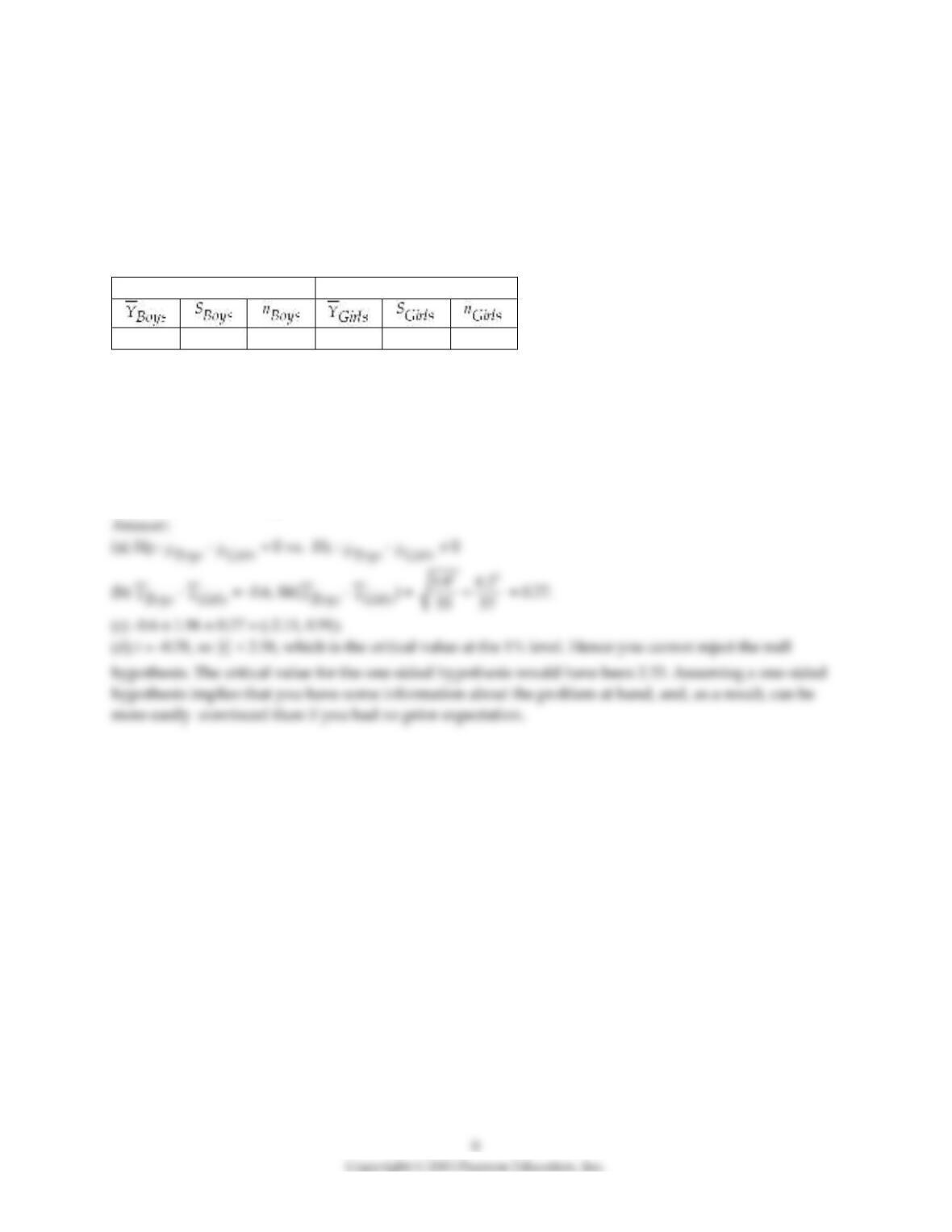
accompanying table shows her findings.
Height of Young Boys and Girls, Grades 4–6, in inches
Boys
Girls
57.8
3.9
55
58.4
4.2
57
(a) Let your null hypothesis be that there is no difference in the height of females and males at this age
level. Specify the alternative hypothesis.
(b) Find the difference in height and the standard error of the difference.
(c) Generate a 95% confidence interval for the difference in height.
(d) Calculate the t–statistic for comparing the two means. Is the difference statistically significant at the
1% level? Which critical value did you use? Why would this number be smaller if you had assumed a
one–sided alternative hypothesis? What is the intuition behind this?
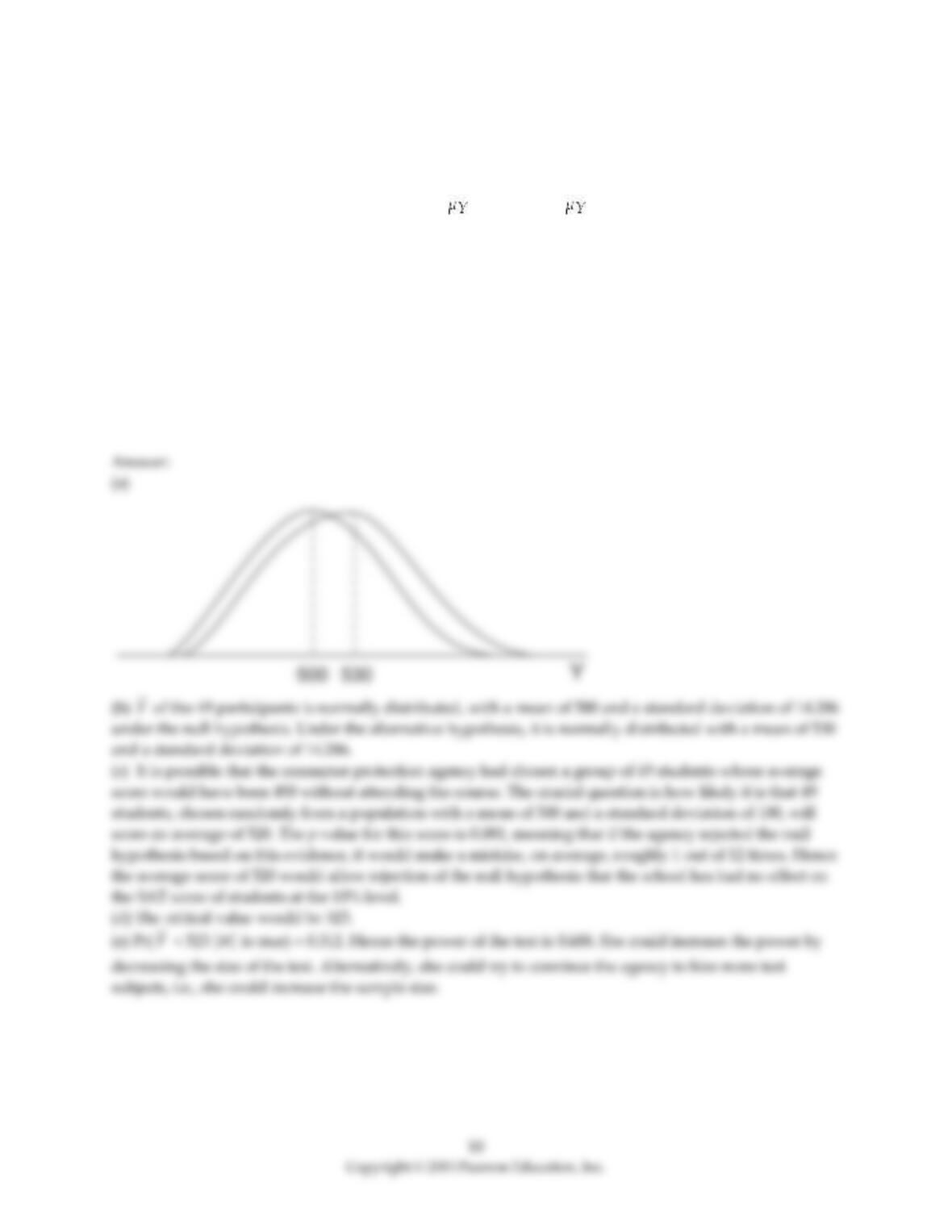
3) Math SAT scores (Y) are normally distributed with a mean of 500 and a standard deviation of 100. An
evening school advertises that it can improve students’ scores by roughly a third of a standard deviation,
or 30 points, if they attend a course which runs over several weeks. (A similar claim is made for attending
a verbal SAT course.) The statistician for a consumer protection agency suspects that the courses are not
effective. She views the situation as follows: H0 : = 500 vs. H1 : = 530.
(a) Sketch the two distributions under the null hypothesis and the alternative hypothesis.
(b) The consumer protection agency wants to evaluate this claim by sending 50 students to attend classes.
One of the students becomes sick during the course and drops out. What is the distribution of the average
score of the remaining 49 students under the null, and under the alternative hypothesis?
(c) Assume that after graduating from the course, the 49 participants take the SAT test and score an
average of 520. Is this convincing evidence that the school has fallen short of its claim? What is the p–
value for such a score under the null hypothesis?
(d) What would be the critical value under the null hypothesis if the size of your test were 5%?
(e) Given this critical value, what is the power of the test? What options does the statistician have for
increasing the power in this situation?
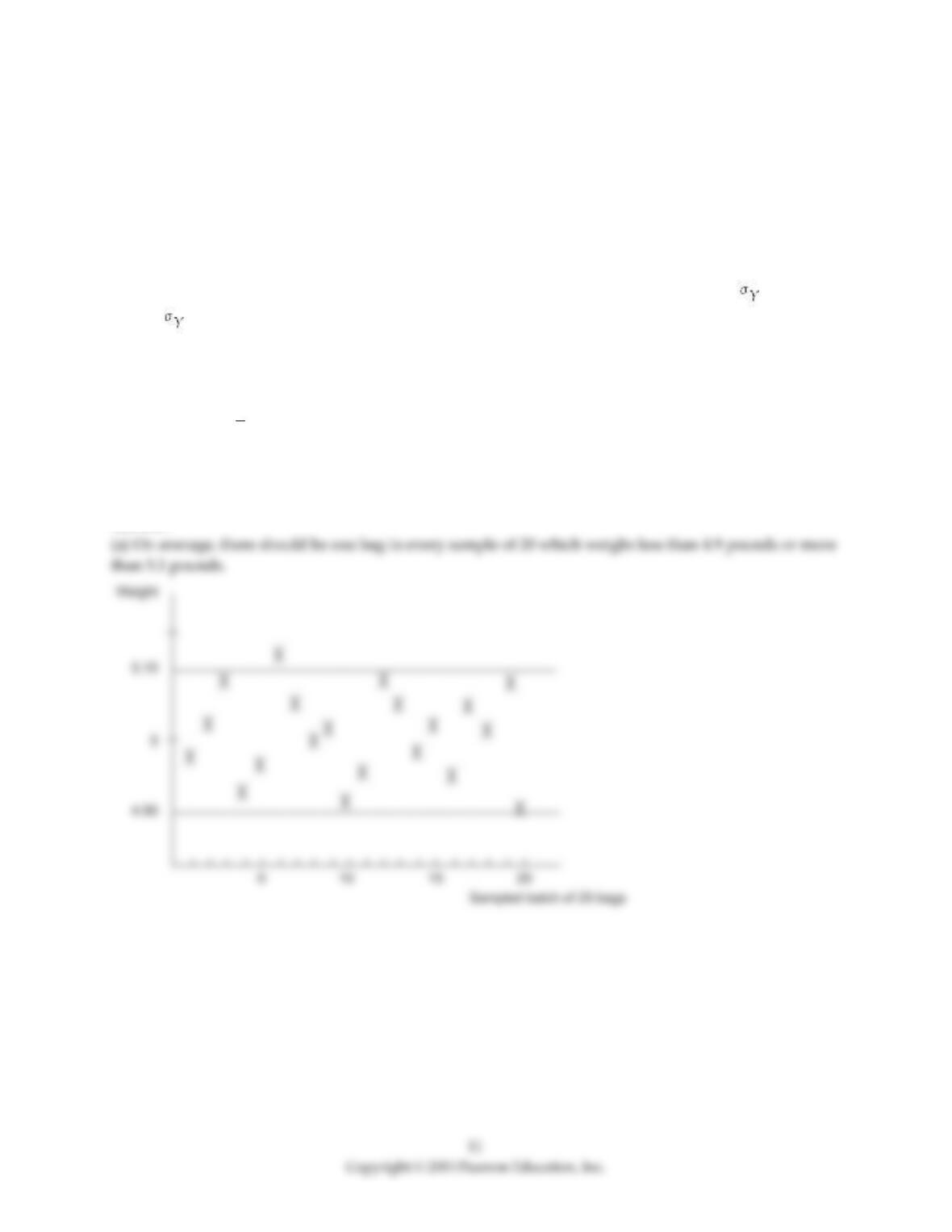
4) Your packaging company fills various types of flour into bags. Recently there have been complaints
from one chain of stores: a customer returned one opened 5 pound bag which weighed significantly less
than the label indicated. You view the weight of the bag as a random variable which is normally
distributed with a mean of 5 pounds, and, after studying the machine specifications, a standard deviation
of 0.05 pounds.
(a) You take a sample of 20 bags and weigh them. Sketch below what the average pattern of individual
weights might look like. Let the horizontal axis indicate the sampled bag number (1, 2, …, 20). On the
vertical axis, mark the expected value of the weight under the null hypothesis, and two (≈ 1.96) standard
deviations above and below the expected value. Draw a line through the graph for E(Y) + 2 , E(Y), and
E(Y) – 2 . How many of the bags in a sample of 20 will you expect to weigh either less than 4.9 pounds
or more than 5.1 pounds?
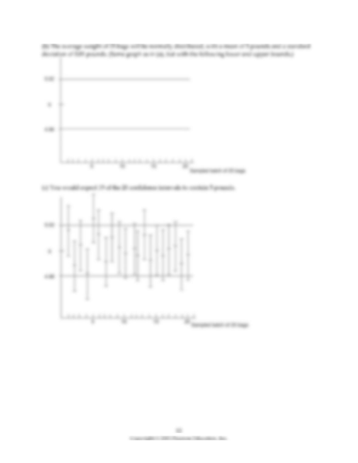
(b) You sample 25 bags of flour and calculate the average weight. What is the distribution of the average
weight of these 25 bags? Repeating the same exercise 20 times, sketch what the distribution of the average
weights would look like in a graph similar to the one you drew in (b), where you have adjusted the
standard error of
Y
accordingly.
(c) For each of the twenty observations in (c) a 95% confidence interval is constructed. Draw these
confidence intervals, using the same graph as in (c). How many of these 20 confidence intervals would
you expect to weigh 5 pounds under the null hypothesis?
Answer:
5) Assume that two presidential candidates, call them Bush and Gore, receive 50% of the votes in the
population. You can model this situation as a Bernoulli trial, where Y is a random variable with success
probability Pr(Y = 1) = p, and where Y = 1 if a person votes for Bush and Y = 0 otherwise. Furthermore, let
ˆ
p
be the fraction of successes (1s) in a sample, which is distributed N(p,
( )
1pp
n
−
) in reasonably large
samples, say for n ≥ 40.
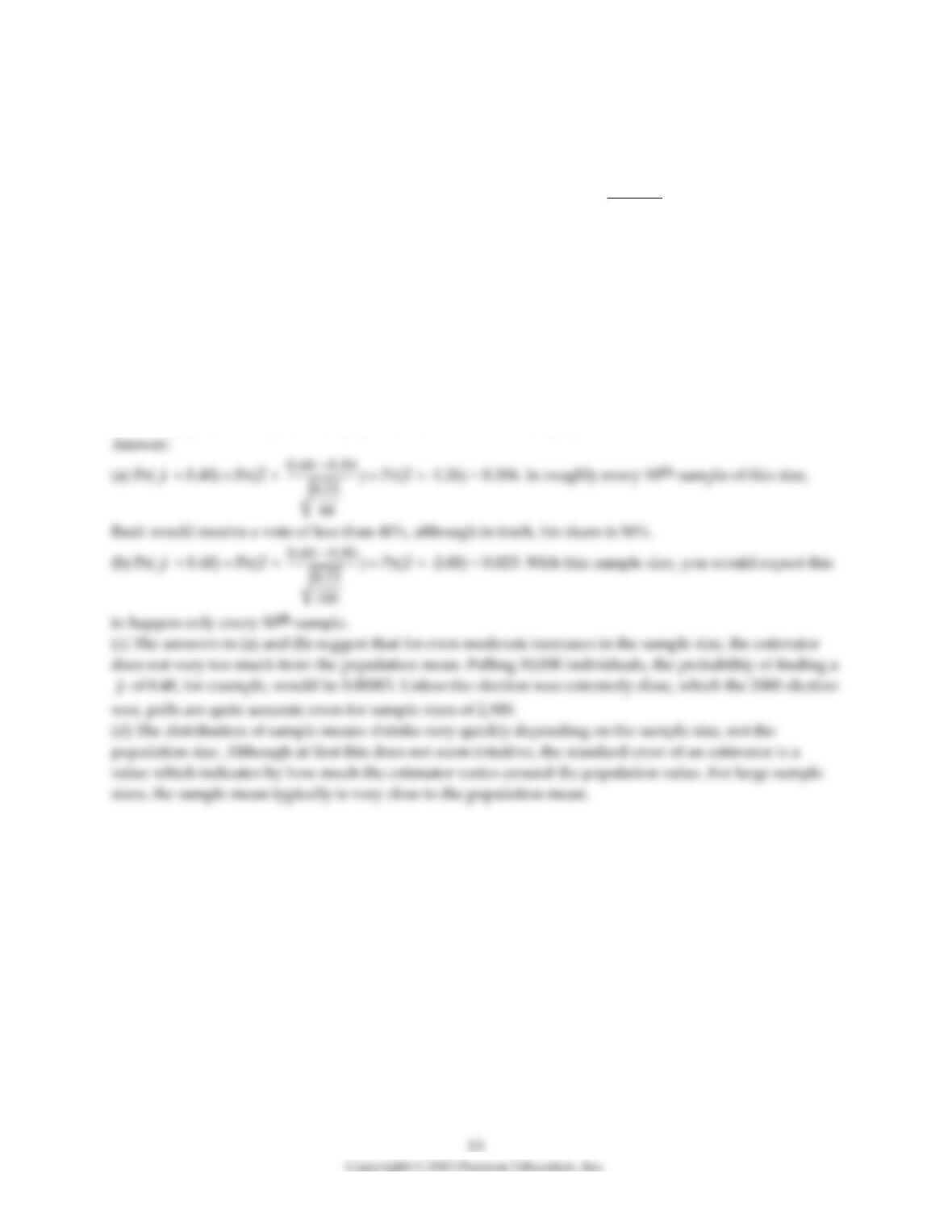
(a) Given your knowledge about the population, find the probability that in a random sample of 40, Bush
would receive a share of 40% or less.
(b) How would this situation change with a random sample of 100?
(c) Given your answers in (a) and (b), would you be comfortable to predict what the voting intentions for
the entire population are if you did not know p but had polled 10,000 individuals at random and
calculated
ˆ
p
? Explain.
(d) This result seems to hold whether you poll 10,000 people at random in the Netherlands or the United
States, where the former has a population of less than 20 million people, while the United States is 15
times as populous. Why does the population size not come into play?
ˆ
p
ˆ
p
6) You have collected weekly earnings and age data from a sub–sample of 1,744 individuals using the
Current Population Survey in a given year.
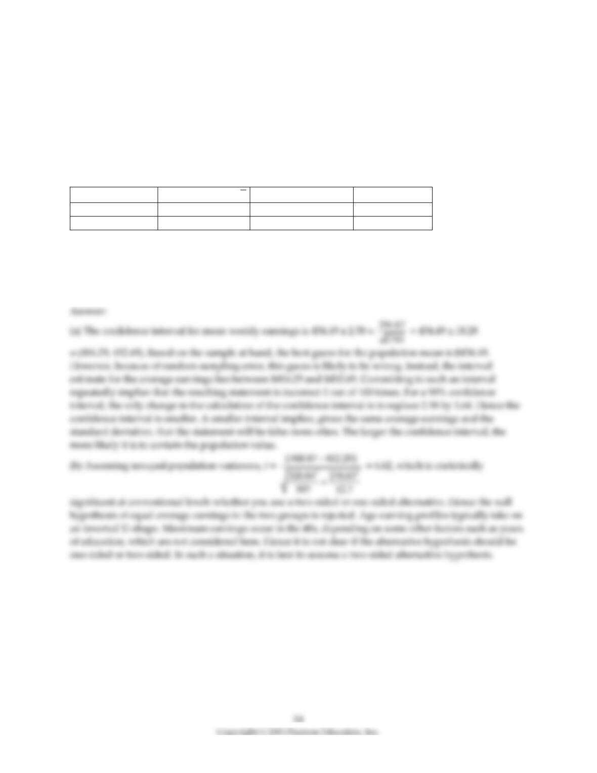
(a) Given the overall mean of $434.49 and a standard deviation of $294.67, construct a 99% confidence
interval for average earnings in the entire population. State the meaning of this interval in words, rather
than just in numbers. If you constructed a 90% confidence interval instead, would it be smaller or larger?
What is the intuition?
(b) When dividing your sample into people 45 years and older, and younger than 45, the information
shown in the table is found.
Age Category
Average Earnings
Y
Standard Deviation
Y
S
N
Age ≥ 45
$488.87
$328.64
507
Age < 45
$412.20
$276.63
1237
Test whether or not the difference in average earnings is statistically significant. Given your knowledge
of age–earning profiles, does this result make sense?
15
7) A manufacturer claims that a certain brand of VCR player has an average life expectancy of 5 years and
6 months with a standard deviation of 1 year and 6 months. Assume that the life expectancy is normally
distributed.
(a) Selecting one VCR player from this brand at random, calculate the probability of its life expectancy
exceeding 7 years.
(b) The Critical Consumer magazine decides to test fifty VCRs of this brand. The average life in this sample
is 6 years and the sample standard deviation is 2 years. Calculate a 99% confidence interval for the
average life.
(c) How many more VCRs would the magazine have to test in order to halve the width of the confidence
interval?
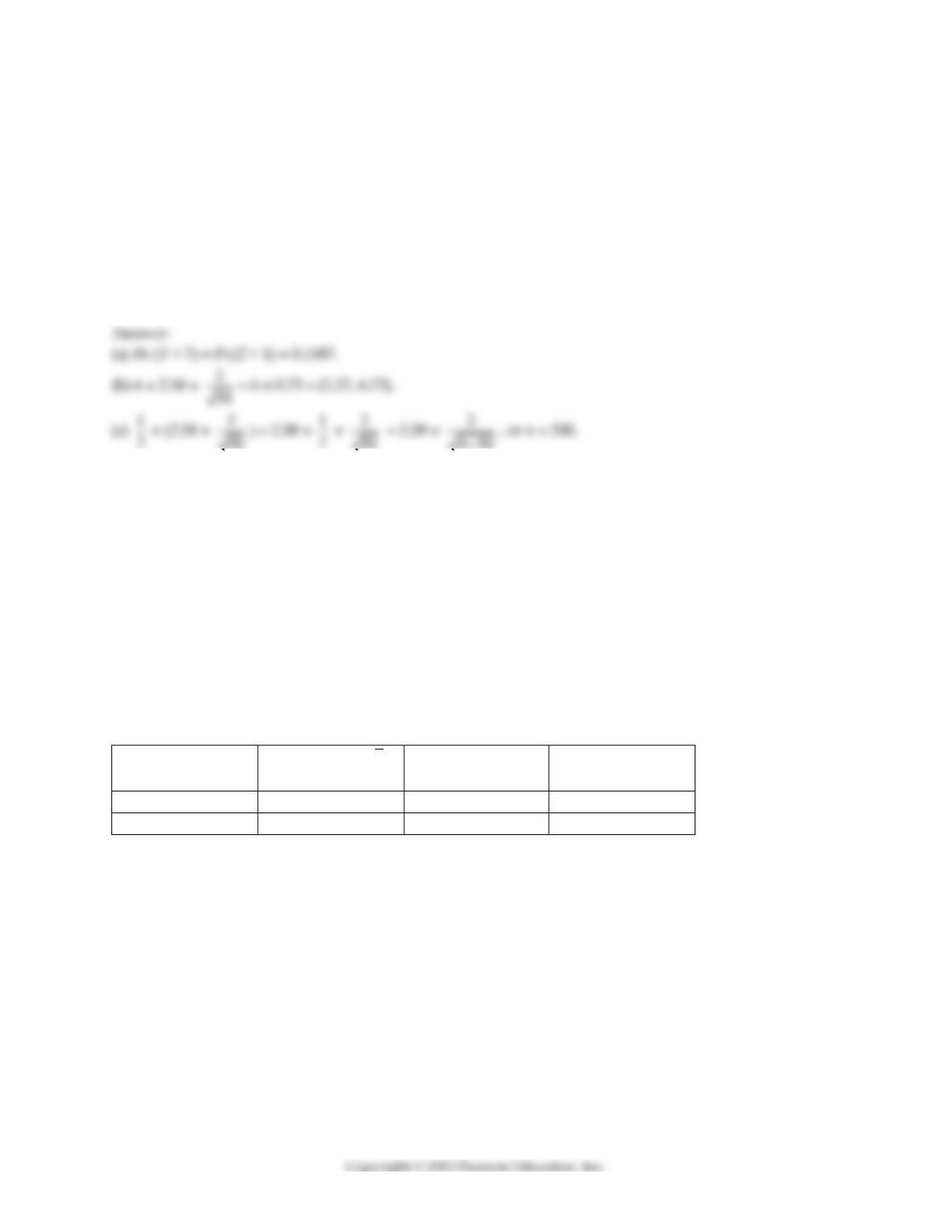
8) U.S. News and World Report ranks colleges and universities annually. You randomly sample 100 of the
national universities and liberal arts colleges from the year 2000 issue. The average cost, which includes
tuition, fees, and room and board, is $23,571.49 with a standard deviation of $7,015.52.
(a) Based on this sample, construct a 95% confidence interval of the average cost of attending a
university/college in the United States.
(b) Cost varies by quite a bit. One of the reasons may be that some universities/colleges have a better
reputation than others. U.S. News and World Reports tries to measure this factor by asking university
presidents and chief academic officers about the reputation of institutions. The ranking is from 1
(“marginal”) to 5 (“distinguished”). You decide to split the sample according to whether the academic
institution has a reputation of greater than 3.5 or not. For comparison, in 2000, Caltech had a reputation
ranking of 4.7, Smith College had 4.5, and Auburn University had 3.1. This gives you the statistics shown
in the accompanying table.
Reputation
Category
Average Cost
Y
Standard deviation
of Cost (
Y
S
)
N
Ranking > 3.5
$29,311.31
$5,649.21
29
Ranking ≤ 3.5
$21,227.06
$6,133.38
71
Test the hypothesis that the average cost for all universities/colleges is the same independent of the
reputation. What alternative hypothesis did you use?
(c) What other factors should you consider before making a decision based on the data in (b)?
9) The development office and the registrar have provided you with anonymous matches of starting
salaries and GPAs for 108 graduating economics majors. Your sample contains a variety of jobs, from
church pastor to stockbroker.
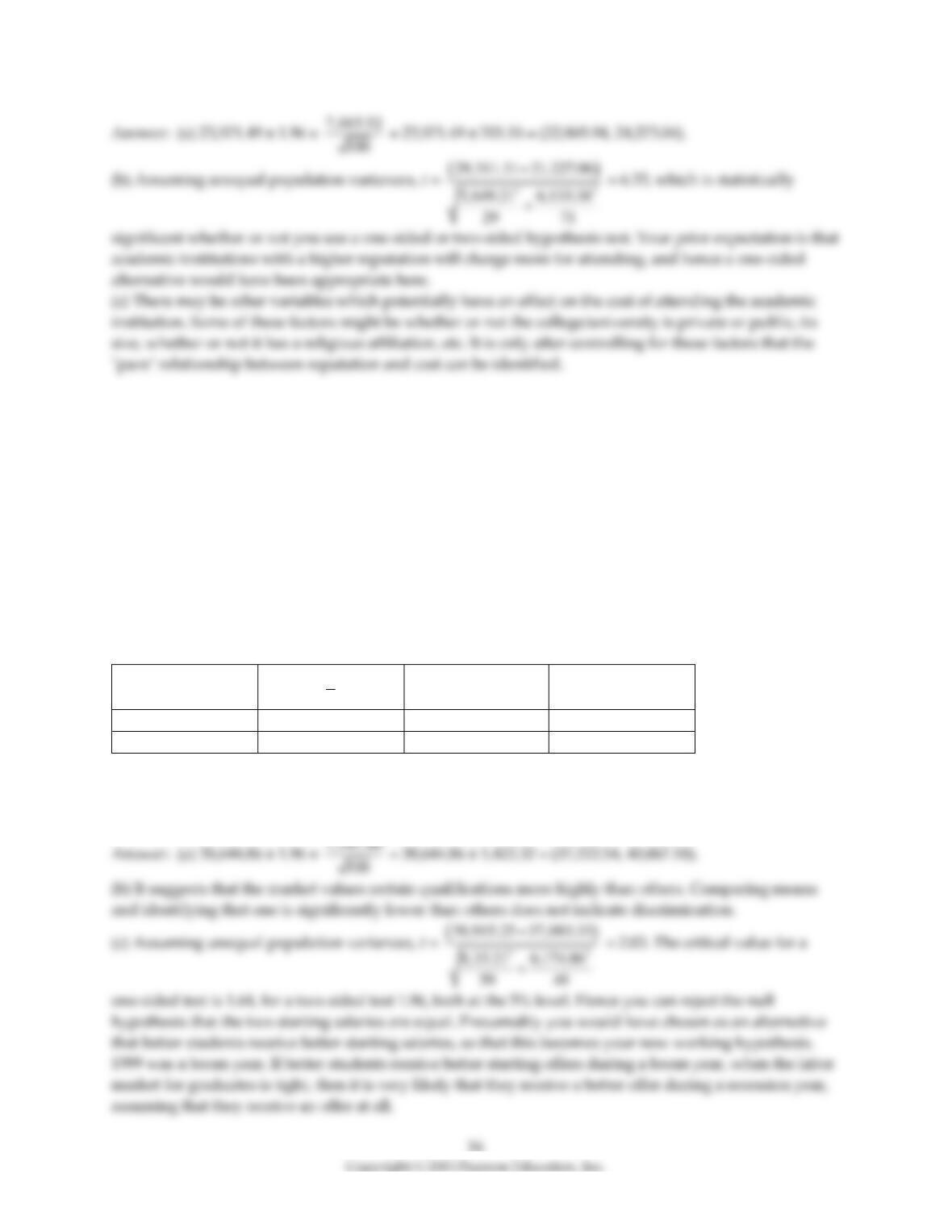
(a) The average starting salary for the 108 students was $38,644.86 with a standard deviation of $7,541.40.
Construct a 95% confidence interval for the starting salary of all economics majors at your
university/college.
(b) A similar sample for psychology majors indicates a significantly lower starting salary. Given that
these students had the same number of years of education, does this indicate discrimination in the job
market against psychology majors?
(c) You wonder if it pays (no pun intended) to get good grades by calculating the average salary for
economics majors who graduated with a cumulative GPA of B+ or better, and those who had a B or
worse. The data is as shown in the accompanying table.
Cumulative GPA
Average Earnings
Y
Standard deviation
Y
S
n
B+ or better
$39,915.25
$8,330.21
59
B or worse
$37,083.33
$6,174.86
49
Conduct a t–test for the hypothesis that the two starting salaries are the same in the population. Given
that this data was collected in 1999, do you think that your results will hold for other years, such as 2002?