Subjective Short Answer
Scenario 21-4 Frank spends all of his income of $240 per month on shirts and hats. The price of a shirt is $40 and the
price of a hat is $30.
1. Refer to Scenario 21-4. If Frank uses all of his income to buy hats during a certain month, then how many hats does he
buy?
2. Refer to Scenario 21-4. If Frank buys 3 shirts during a certain month, then how many hats does he buy during that
month?
3. Refer to Scenario 21-4. What is the slope of Frank’s budget constraint if it is drawn with the quantity of shirts on the
horizontal axis and the quantity of hats on the vertical axis?
Figure 21–30 The graph shows two budget constraints for a consumer.
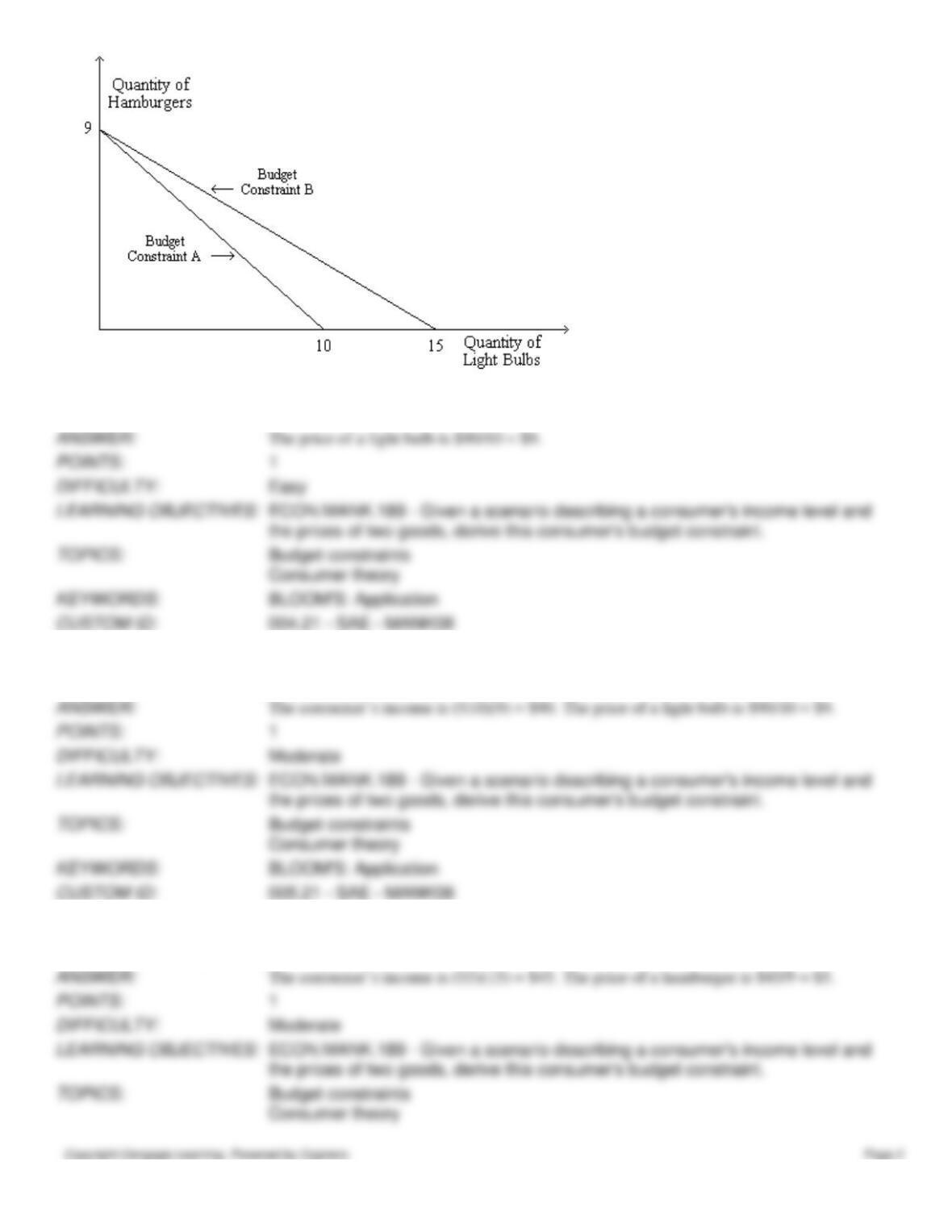
4. Refer to Figure 21–30. Suppose the consumer’s income is $90 and Budget Constraint A applies. What is the price of a
light bulb?
5. Refer to Figure 21–30. Suppose the price of a hamburger is $10 and Budget Constraint A applies. What is the
consumer’s income? What is the price of a light bulb?
6. Refer to Figure 21–30. Suppose the price of a light bulb is $3 and Budget Constraint B applies. What is the consumer’s
income? What is the price of a hamburger?
7. Refer to Figure 21–30. What particular change would result in a rotation of the budget constraint from Budget
Constraint A to Budget Constraint B?
8. Refer to Figure 21–30. Suppose Budget Constraint B applies. If the consumer’s income is $90 and if he is buying 5
light bulbs, then how much money is he spending on hamburgers?
9. If the market is offering consumers the trade-off of 3 pints of Pepsi for 1 pizza, and if the price of a pizza is $9, then
what is the price of a pint of Pepsi?
10. A consumer’s budget constraint is drawn with the quantity of pizza measured along the horizontal axis and the price of
Pepsi measured along the vertical axis. If the market is offering the consumer the trade-off of 3 pints of Pepsi for 1 pizza,
then what is the slope of the consumer’s budget constraint?
11. What does the slope of a budget constraint represent?
12. A consumer’s budget constraint is drawn on a graph with the number of sandwiches measured along the horizontal
axis and the number of bowls of soup measured along the vertical axis. Hold the consumer’s income and the price of a
sandwich fixed, and increase the price of a bowl of soup. Describe the effect on the budget constraint.
13. The rate at which a consumer is willing to trade off one good for another is called the __________.
14. In order to represent a consumer’s choices on a graph, we draw her budget constraint as well as her __________
curves.
15. When we draw Katie’s indifference curves to represent her preferences for books and movies, we find that her
indifference curves are upward-sloping. What does this tell us about Katie’s preferences?
16. A consumer’s indifference curves are right angles when, for the consumer, the goods in question are __________.
17. A consumer’s indifference curves are straight lines when, for the consumer, the goods in question are __________.
18. What does the slope of a consumer’s indifference curve represent?
19. Because people are more willing to trade away goods that they have in abundance and less willing to trade away
goods of which they have little, indifference curves are ___________.
20. Teresa faces prices of $6.00 for a unit of good X and $1.50 for a unit of good Y. At her optimum, Teresa is willing to
give up 1 unit of good X for __________ units of good Y.
21. Thomas faces prices of $6 for a unit of good X and $30 for a unit of good Y. At his optimum, Thomas is willing to
give up 1 unit of good Y for __________ units of good X.
22. If goods X and Y are both normal goods for Brenda, then an increase in Brenda’s income will lead her to __________.
23. Using our model of consumer choice, is it possible for a consumer to buy less of a particular good when his income
rises? Briefly explain.
24. What is significant about a point on a graph at which an indifference curve is tangent to a budget constraint?
25. Goods x and y are available to Jeff. At Jeff’s optimum, the marginal utility per dollar spent on good x equals
__________________.
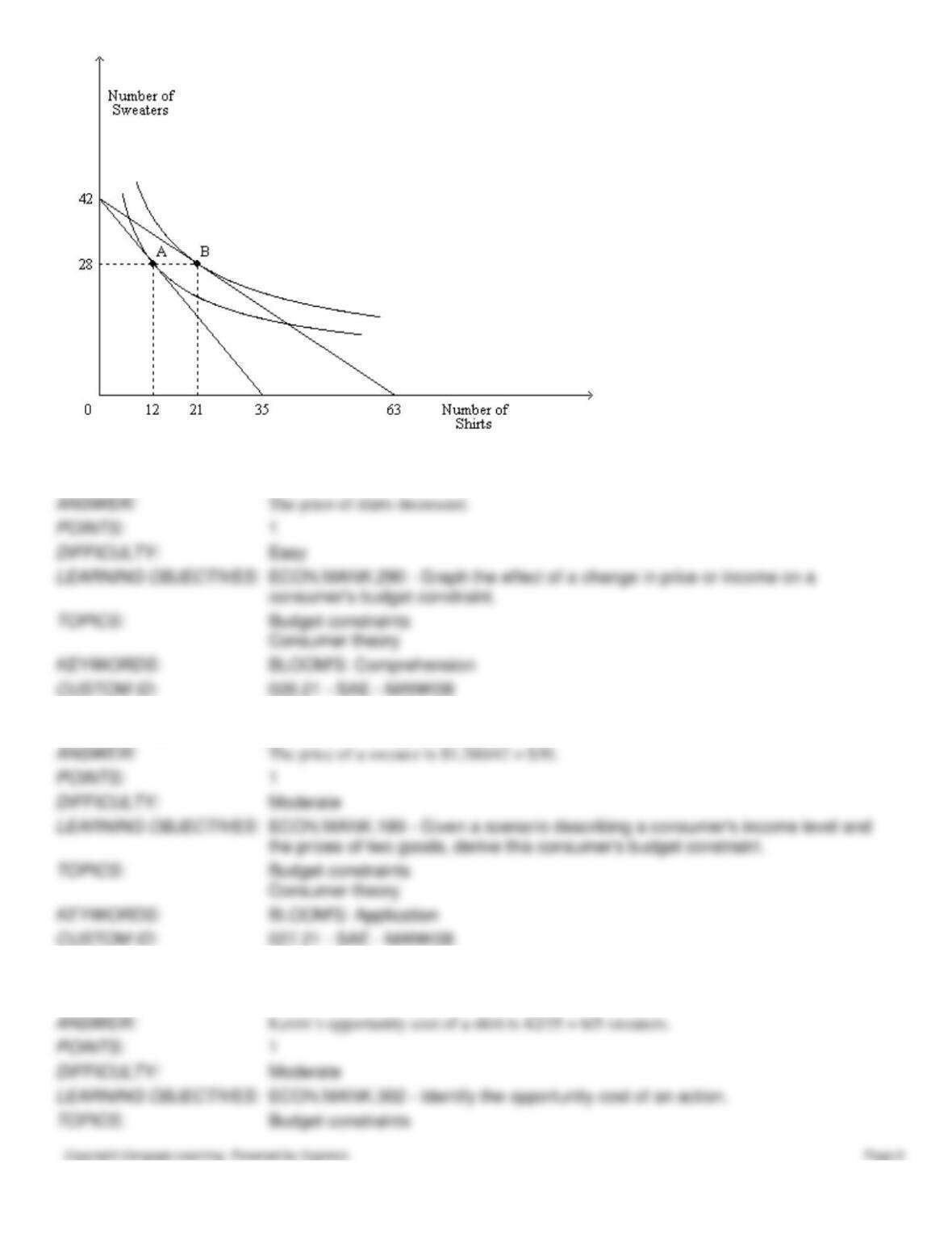
26. Refer to Figure 21–31. Suppose point A was Kevin’s optimum last week, and point B is his optimum this week. What
happened between last week and this week?
27. Refer to Figure 21–31. If Kevin’s income is $1,260, then what is the price of a sweater?
28. Refer to Figure 21–31. If point A is Kevin’s optimum, then at that optimum, what is his opportunity cost of a shirt in
terms of sweaters?
29. Refer to Figure 21–31. If the price of a shirt is $36 and point A is Kevin’s optimum, then what is Kevin’s income?
30. Refer to Figure 21–31. If Kevin’s income is $1,260 and point A is his optimum, then what is the price of a shirt?
31. Refer to Figure 21–31. Suppose Kevin is optimally purchasing 12 shirts and 28 sweaters, and he is spending $648 on
shirts. What is the price of a sweater?
32. Refer to Figure 21–31. Suppose Kevin is optimally purchasing 21 shirts and 28 sweaters, and he is spending $1,680
on sweaters. What is the price of a shirt?
33. Refer to Figure 21–31. If point B is Kevin’s optimum, then at that optimum, what is his opportunity cost of a sweater
in terms of shirts?
34. Refer to Figure 21–31. If the price of a shirt is $20 and point B is Kevin’s optimum, then what is Kevin’s income?
35. Refer to Figure 21–31. If Kevin’s income is $2,520 and point B is his optimum, then what is the price of a shirt?
36. Refer to Figure 21–31. For Kevin, are sweaters and shirts substitutes, complements, or neither?
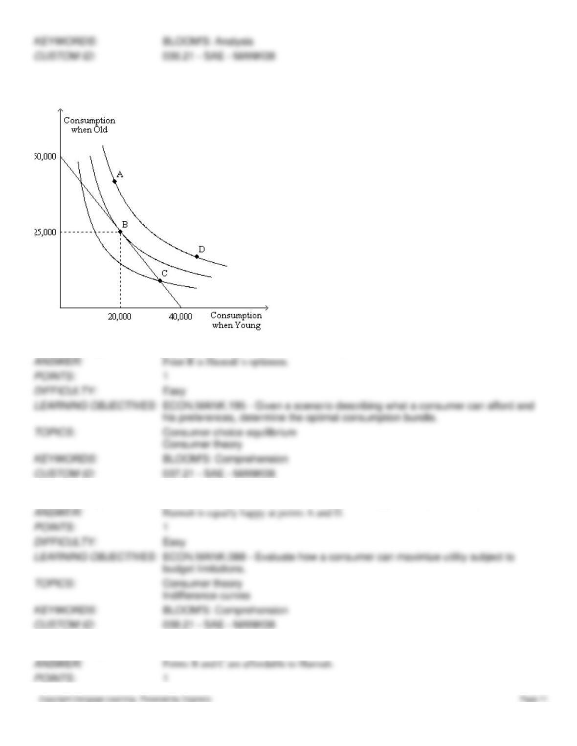
Figure 21–32 The figure shows three indifference curves and a budget constraint for a consumer named Hannah. When
young, Hannah works and earns income. When old, she is retired and earns no income.
37. Refer to Figure 21–32. Which of the four labeled points is Hannah’s optimum?
38. Refer to Figure 21–32. At two of the four labeled points, Hannah is equally happy. Identify those two points.
39. Refer to Figure 21–32. Of the four labeled points, which is (are) affordable to Hannah?