Introduction to Econometrics, 3e (Stock)
Chapter 2 Review of Probability
2.1 Multiple Choice
1) The probability of an outcome
A) is the number of times that the outcome occurs in the long run.
B) equals M × N, where M is the number of occurrences and N is the population size.
C) is the proportion of times that the outcome occurs in the long run.
D) equals the sample mean divided by the sample standard deviation.
2) The probability of an event A or B (Pr(A or B)) to occur equals
A) Pr(A) × Pr(B).
B) Pr(A) + Pr(B) if A and B are mutually exclusive.
C)
( )
( )
Pr
Pr
A
B
.
D) Pr(A) + Pr(B) even if A and B are not mutually exclusive.
3) The cumulative probability distribution shows the probability
A) that a random variable is less than or equal to a particular value.
B) of two or more events occurring at once.
C) of all possible events occurring.
D) that a random variable takes on a particular value given that another event has happened.
4) The expected value of a discrete random variable
A) is the outcome that is most likely to occur.
B) can be found by determining the 50% value in the c.d.f.
C) equals the population median.
D) is computed as a weighted average of the possible outcome of that random variable, where the
weights are the probabilities of that outcome.
5) Let Y be a random variable. Then var(Y) equals
A)
2
)
Y
EY
−
.
B)
( )
Y
EY
−
.
C)
( )
2
Y
EY
−
.
D)
( )
Y
EY
−
.

6) The skewness of the distribution of a random variable Y is defined as follows:
A)
( )
3
2
Y
Y
EY
−
B)
( )
3
Y
EY
−
C)
( )
33
3
Y
Y
EY
−
D)
( )
3
3
Y
Y
EY
−
7) The skewness is most likely positive for one of the following distributions:
A) The grade distribution at your college or university.
B) The U.S. income distribution.
C) SAT scores in English.
D) The height of 18 year old females in the U.S.
8) The kurtosis of a distribution is defined as follows:
A)
( )
4
4
Y
Y
EY
−
B)
( )
44
2
Y
Y
EY
−
C)
var( )
skewness
Y
D) E[(Y – )4)
9) For a normal distribution, the skewness and kurtosis measures are as follows:
A) 1.96 and 4
B) 0 and 0
C) 0 and 3
D) 1 and 2

10) The conditional distribution of Y given X = x, Pr(Y = y=x), is
A)
( )
( )
Pr
Pr
Yy
Xx
=
=
.
B)
( )
1
Pr ,
l
i
i
X x Y y
=
==
C)
( )
( )
Pr ,
Pr
X x Y y
Yy
==
=
D)
( )
( )
Pr ,
Pr
X x Y y
Xx
==
=
.
11) The conditional expectation of Y given X, E(Y, is calculated as follows:
A)
( )
1
Pr
k
ii
i
Y X x Y y
=
==
B) E
C)
( )
1
Pr
k
ii
i
y Y y X x
=
==
D)
( )
( )
1
Pr
k
ii
i
E Y X x X x
=
==
12) Two random variables X and Y are independently distributed if all of the following conditions hold,
with the exception of
A) Pr(Y = y = x) = Pr(Y = y).
B) knowing the value of one of the variables provides no information about the other.
C) if the conditional distribution of Y given X equals the marginal distribution of Y.
D) E(Y) = E[E(Y)].
13) The correlation between X and Y
A) cannot be negative since variances are always positive.
B) is the covariance squared.
C) can be calculated by dividing the covariance between X and Y by the product of the two standard
deviations.
D) is given by corr(X, Y) =
( )
( ) ( )
cov ,
var var
XY
XY
.
14) Two variables are uncorrelated in all of the cases below, with the exception of
A) being independent.
B) having a zero covariance.
C)
22
XY
XY
D) E(Y ) = 0.
15) var(aX + bY) =
A)
B)
C)
D)
16) To standardize a variable you
A) subtract its mean and divide by its standard deviation.
B) integrate the area below two points under the normal distribution.
C) add and subtract 1.96 times the standard deviation to the variable.
D) divide it by its standard deviation, as long as its mean is 1.
17) Assume that Y is normally distributed N(μ, σ2). Moving from the mean (μ) 1.96 standard deviations to
the left and 1.96 standard deviations to the right, then the area under the normal p.d.f. is
A) 0.67
B) 0.05
C) 0.95
D) 0.33
18) Assume that Y is normally distributed N(μ, σ2). To find Pr(c1 ≤ Y ≤ c2), where c1 < c2 and di =
i
c
−
,
you need to calculate Pr(d1 ≤ Z ≤ d2) =
A) Φ(d2) – Φ(d1)
B) Φ(1.96) – Φ(1.96)
C) Φ(d2) – (1 – Φ(d1))
D) 1 – (Φ(d2) – Φ(d1))
19) If variables with a multivariate normal distribution have covariances that equal zero, then
A) the correlation will most often be zero, but does not have to be.
B) the variables are independent.
C) you should use the χ2 distribution to calculate probabilities.
D) the marginal distribution of each of the variables is no longer normal.
20) The Student t distribution is
A) the distribution of the sum of m squared independent standard normal random variables.
B) the distribution of a random variable with a chi–squared distribution with m degrees of freedom,
divided by m.
C) always well approximated by the standard normal distribution.
D) the distribution of the ratio of a standard normal random variable, divided by the square root of an
independently distributed chi–squared random variable with m degrees of freedom divided by m.
21) When there are ∞ degrees of freedom, the t∞ distribution
A) can no longer be calculated.
B) equals the standard normal distribution.
C) has a bell shape similar to that of the normal distribution, but with “fatter” tails.
D) equals the
2
X
distribution.
22) The sample average is a random variable and
A) is a single number and as a result cannot have a distribution.
B) has a probability distribution called its sampling distribution.
C) has a probability distribution called the standard normal distribution.
D) has a probability distribution that is the same as for the Y1,…, Yn i.i.d. variables.
23) To infer the political tendencies of the students at your college/university, you sample 150 of them.
Only one of the following is a simple random sample: You
A) make sure that the proportion of minorities are the same in your sample as in the
entire student body.
B) call every fiftieth person in the student directory at 9 a.m. If the person does not answer the phone,
you pick the next name listed, and so on.
C) go to the main dining hall on campus and interview students randomly there.
D) have your statistical package generate 150 random numbers in the range from 1 to the total number of
students in your academic institution, and then choose the corresponding names in the student telephone
directory.
24) The variance of
2
,YY
, is given by the following formula:
A)
2
Y
.
B)
Y
n
.
C)
2
Y
n
.
D)
2
Y
n
.
25) The mean of the sample average
Y
,
( )
EY
, is
A)
1
Y
n
.
B)
Y
.
C)
Y
n
.
D)
Y
Y
for n > 30.
26) In econometrics, we typically do not rely on exact or finite sample distributions because
A) we have approximately an infinite number of observations (think of re–sampling).
B) variables typically are normally distributed.
C) the covariances of Yi, Yj are typically not zero.
D) asymptotic distributions can be counted on to provide good approximations to the exact sampling
distribution (given the number of observations available in most cases).
27) Consistency for the sample average
Y
can be defined as follows, with the exception of
A)
Y
converges in probability to
Y
.
B)
Y
has the smallest variance of all estimators.
C)
p
Y
Y
⎯⎯→
.
D) the probability of
Y
being in the range
Y
± c becomes arbitrarily close to one as n increases for any
constant c > 0.
28) The central limit theorem states that
A) the sampling distribution of
Y
Y
Y
−
is approximately normal.
B)
p
Y
Y
⎯⎯→
.
C) the probability that
Y
is in the range
Y
± c becomes arbitrarily close to one as n increases for any
constant c > 0.
D) the t distribution converges to the F distribution for approximately n > 30.
29) The central limit theorem
A) states conditions under which a variable involving the sum of Y1,…, Yn i.i.d. variables becomes the
standard normal distribution.
B) postulates that the sample mean
Y
is a consistent estimator of the population mean
Y
.
C) only holds in the presence of the law of large numbers.
D) states conditions under which a variable involving the sum of Y1,…, Yn i.i.d. variables becomes the
Student t distribution.
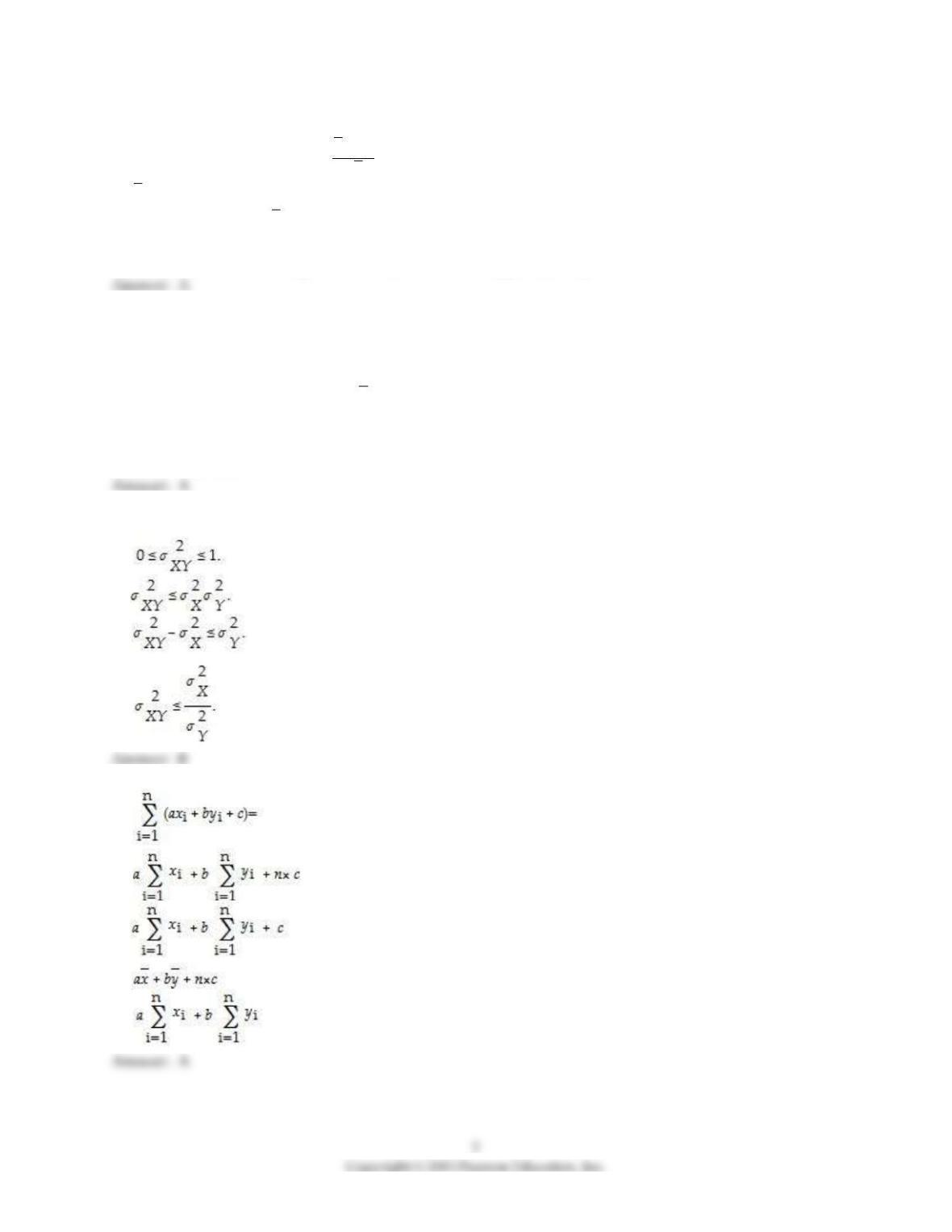
30) The covariance inequality states that
A)
B)
C)
D)
31)
A)
B)
C)
D)

32)
( )
1
n
i
i
ax b
=
+
A) n × a ×
x
+ n × b
B) n(a + b)
C)
x n b+
D)
n a x
33) Assume that you assign the following subjective probabilities for your final grade in your
econometrics course (the standard GPA scale of 4 = A to 0 = F applies):
Grade
Probability
A
0.20
B
0.50
C
0.20
D
0.08
F
0.02
The expected value is:
A) 3.0
B) 3.5
C) 2.78
D) 3.25
34) The mean and variance of a Bernoille random variable are given as
A) cannot be calculated
B) np and np(1–p)
C) p and
( )
1pp−
D) p and (1– p)
35) Consider the following linear transformation of a random variable y =
x
x
x
−
where μx is the mean of
x and σx is the standard deviation. Then the expected value and the standard deviation of Y are given as
A) 0 and 1
B) 1 and 1
C) Cannot be computed because Y is not a linear function of X
D)
x
and σx
2.2 Essays and Longer Questions
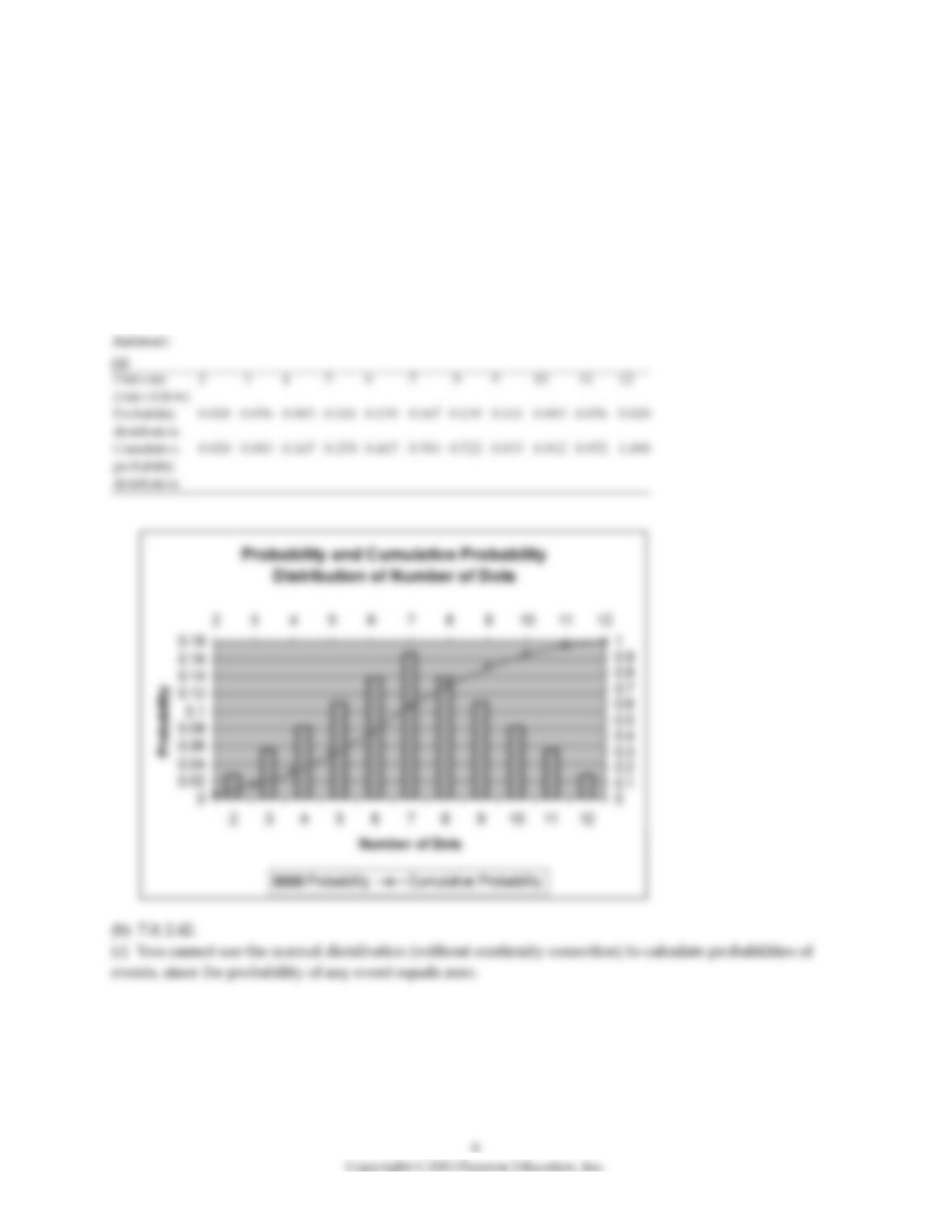
1) Think of the situation of rolling two dice and let M denote the sum of the number of dots on the two
dice. (So M is a number between 1 and 12.)
(a) In a table, list all of the possible outcomes for the random variable M together with its probability
distribution and cumulative probability distribution. Sketch both distributions.
(b) Calculate the expected value and the standard deviation for M.
(c) Looking at the sketch of the probability distribution, you notice that it resembles a normal distribution.
Should you be able to use the standard normal distribution to calculate probabilities of events? Why or
why not?
2) What is the probability of the following outcomes?
(a) Pr(M = 7)
(b) Pr(M = 2 or M = 10)
(c) Pr(M = 4 or M ≠ 4)
(d) Pr(M = 6 and M = 9)
(e) Pr(M < 8)
(f) Pr(M = 6 or M > 10)
11
3) Probabilities and relative frequencies are related in that the probability of an outcome is the proportion
of the time that the outcome occurs in the long run. Hence concepts of joint, marginal, and conditional
probability distributions stem from related concepts of frequency distributions.
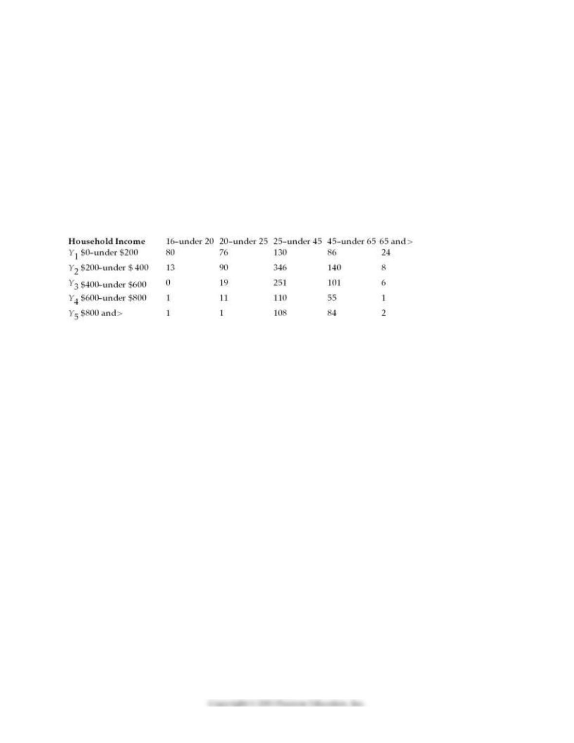
You are interested in investigating the relationship between the age of heads of households and weekly
earnings of households. The accompanying data gives the number of occurrences grouped by age and
income. You collect data from 1,744 individuals and think of these individuals as a population that you
want to describe, rather than a sample from which you want to infer behavior of a larger population.
After sorting the data, you generate the accompanying table:
Joint Absolute Frequencies of Age and Income, 1,744 Households
Age of head of household
X1 X2 X3 X4 X5
The median of the income group of $800 and above is $1,050.
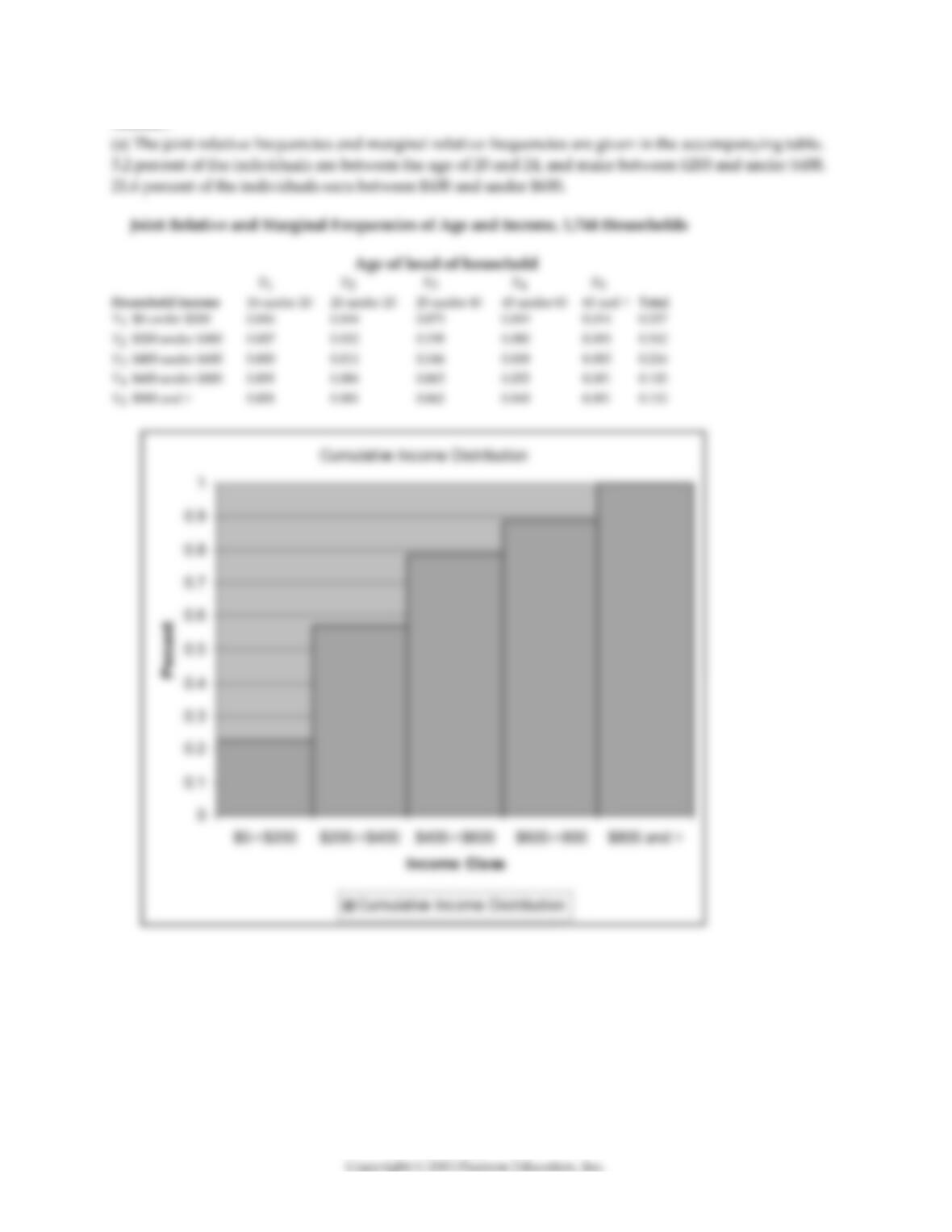
(a) Calculate the joint relative frequencies and the marginal relative frequencies. Interpret one of each of
these. Sketch the cumulative income distribution.
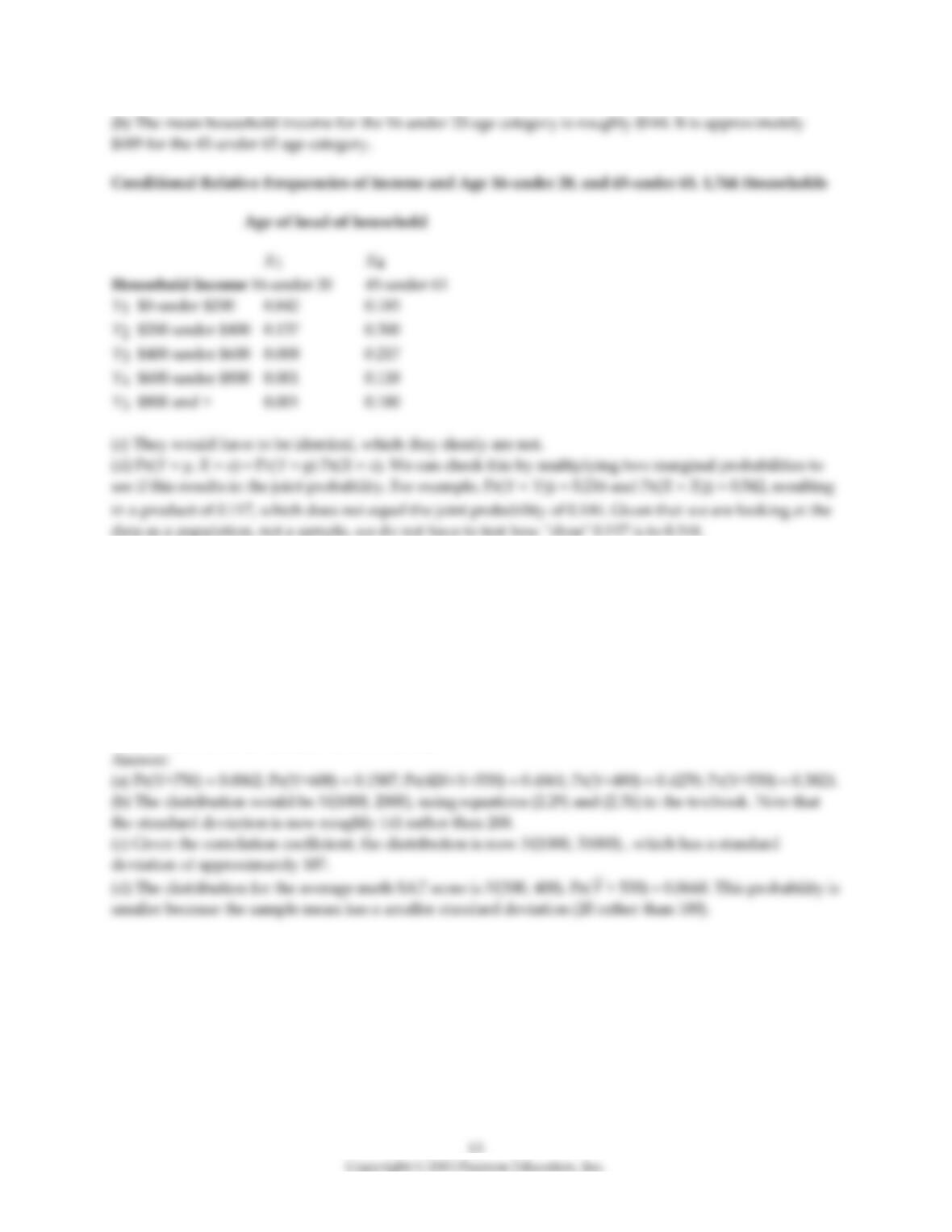
(b) Calculate the conditional relative income frequencies for the two age categories 16–under 20, and 45–
under 65. Calculate the mean household income for both age categories.
(c) If household income and age of head of household were independently distributed, what would you
expect these two conditional relative income distributions to look like? Are they similar here?
(d) Your textbook has given you a primary definition of independence that does not involve conditional
relative frequency distributions. What is that definition? Do you think that age and income are
independent here, using this definition?
12
Answer:
4) Math and verbal SAT scores are each distributed normally with N (500,10000).
(a) What fraction of students scores above 750? Above 600? Between 420 and 530? Below 480? Above 530?
(b) If the math and verbal scores were independently distributed, which is not the case, then what would
be the distribution of the overall SAT score? Find its mean and variance.
(c) Next, assume that the correlation coefficient between the math and verbal scores is 0.75. Find the mean
and variance of the resulting distribution.
(d) Finally, assume that you had chosen 25 students at random who had taken the SAT exam. Derive the
distribution for their average math SAT score. What is the probability that this average is above 530? Why
is this so much smaller than your answer in (a)?
5) The following problem is frequently encountered in the case of a rare disease, say AIDS, when
determining the probability of actually having the disease after testing positively for HIV. (This is often
known as the accuracy of the test given that you have the disease.) Let us set up the problem as follows: Y
= 0 if you tested negative using the ELISA test for HIV, Y = 1 if you tested positive; X = 1 if you have HIV,
X = 0 if you do not have HIV. Assume that 0.1 percent of the population has HIV and that the accuracy of
the test is 0.95 in both cases of (i) testing positive when you have HIV, and (ii) testing negative when you
do not have HIV. (The actual ELISA test is actually 99.7 percent accurate when you have HIV, and 98.5
percent accurate when you do not have HIV.)
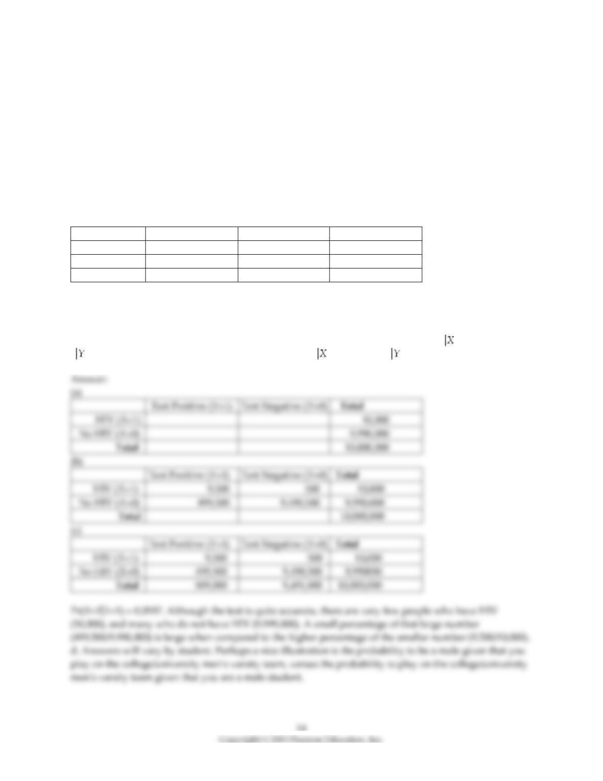
(a) Assuming arbitrarily a population of 10,000,000 people, use the accompanying table to first enter the
column totals.
Test Positive (Y=1)
Test Negative (Y=0)
Total
HIV (X=1)
No HIV (X=0)
Total
10,000,000
(b) Use the conditional probabilities to fill in the joint absolute frequencies.
(c) Fill in the marginal absolute frequencies for testing positive and negative. Determine the conditional
probability of having HIV when you have tested positive. Explain this surprising result.
(d) The previous problem is an application of Bayes’ theorem, which converts Pr(Y = y = x) into Pr(X =
x = y). Can you think of other examples where Pr(Y = y = x) ≠ Pr(X = x = y)?
HIV (X=1)
10,000
No HIV (X=0)
9,990,000
Total
10,000,000
Test Positive (Y=1)
Test Negative (Y=0)
Total
HIV (X=1)
9,500
500
10,000
No HIV (X=0)
499,500
9,490,500
9,990,000
Total
10,000,000
Test Positive (Y=1)
Test Negative (Y=0)
Total
HIV (X=1)
9,500
500
10,000
No HIV (X=0)
499,500
9,490,500
9,990000
Total
509,000
9,491,000
10,000,000
6) You have read about the so–called catch–up theory by economic historians, whereby nations that are
further behind in per capita income grow faster subsequently. If this is true systematically, then
eventually laggards will reach the leader. To put the theory to the test, you collect data on relative (to the
United States) per capita income for two years, 1960 and 1990, for 24 OECD countries. You think of these
countries as a population you want to describe, rather than a sample from which you want to infer
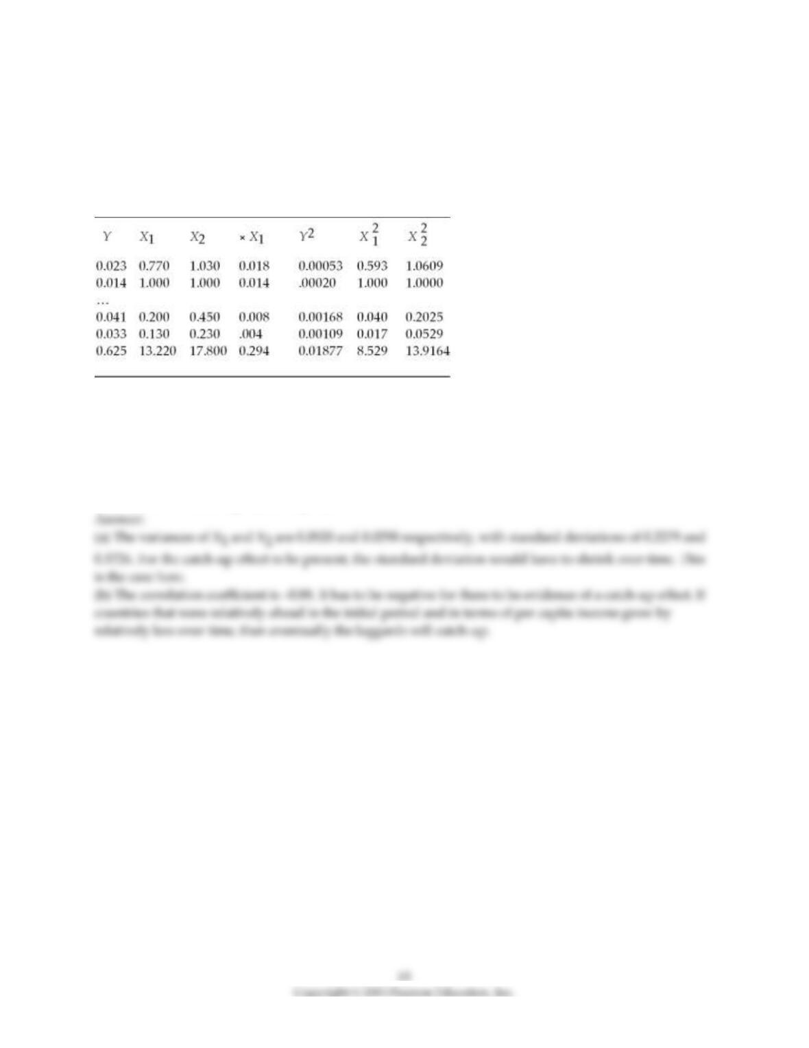
behavior of a larger population. The relevant data for this question is as follows:
where X1 and X2 are per capita income relative to the United States in 1960 and 1990 respectively, and Y
is the average annual growth rate in X over the 1960–1990 period. Numbers in the last row represent sums
of the columns above.
(a) Calculate the variance and standard deviation of X1 and X2. For a catch–up effect to be present, what
relationship must the two standard deviations show? Is this the case here?
(b) Calculate the correlation between Y and . What sign must the correlation coefficient have for there to
be evidence of a catch–up effect? Explain.
7) Following Alfred Nobel’s will, there are five Nobel Prizes awarded each year. These are for
outstanding achievements in Chemistry, Physics, Physiology or Medicine, Literature, and Peace. In 1968,
the Bank of Sweden added a prize in Economic Sciences in memory of Alfred Nobel. You think of the
data as describing a population, rather than a sample from which you want to infer behavior of a larger
population. The accompanying table lists the joint probability distribution between recipients in
economics and the other five prizes, and the citizenship of the recipients, based on the 1969–2001 period.
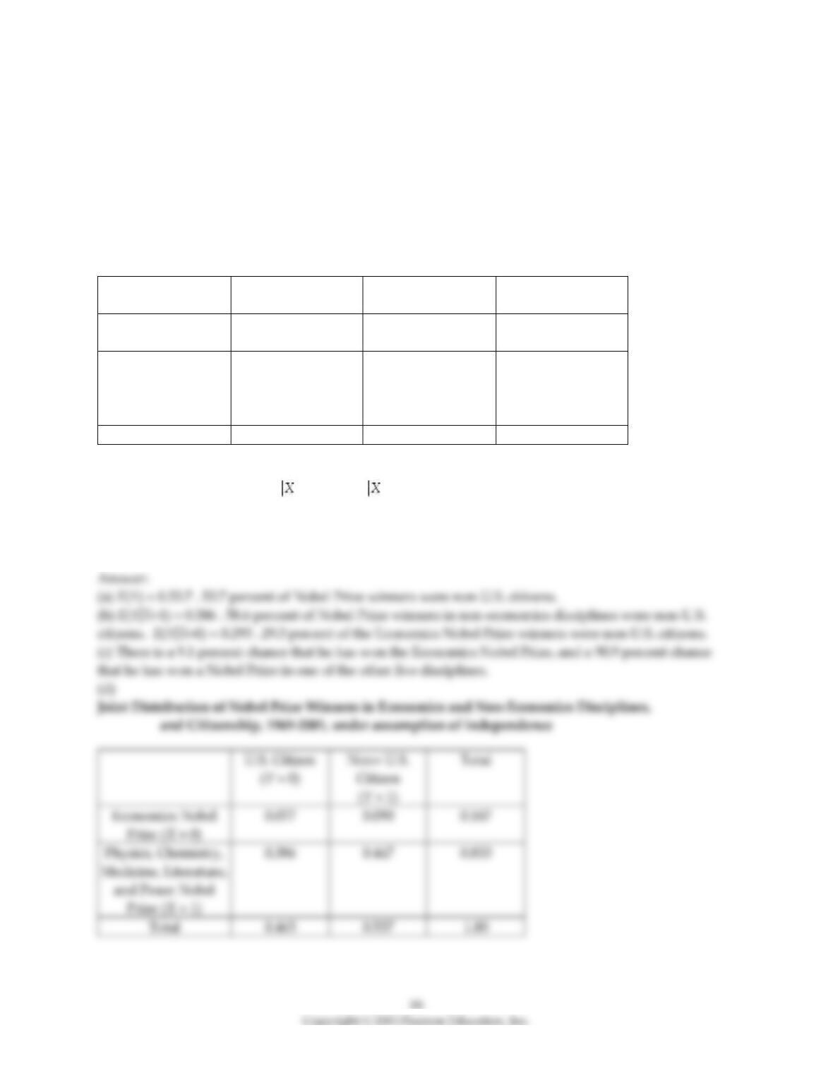
Joint Distribution of Nobel Prize Winners in Economics and Non–Economics
Disciplines, and Citizenship, 1969–2001
U.S. Citizen
(Y = 0)
Non= U.S. Citizen
(Y = 1)
Total
Economics Nobel
Prize (X = 0)
0.118
0.049
0.167
Physics, Chemistry,
Medicine, Literature,
and Peace Nobel
Prize (X = 1)
0.345
0.488
0.833
Total
0.463
0.537
1.00
(a) Compute E(Y) and interpret the resulting number.
(b) Calculate and interpret E(Y=1) and E(Y=0).
(c) A randomly selected Nobel Prize winner reports that he is a non–U.S. citizen. What is the probability
that this genius has won the Economics Nobel Prize? A Nobel Prize in the other five disciplines?
(d) Show what the joint distribution would look like if the two categories were independent.
Economics Nobel
Prize (X = 0)
Physics, Chemistry,
Medicine, Literature,
and Peace Nobel
Prize (X = 1)
Total

17
8) A few years ago the news magazine The Economist listed some of the stranger explanations used in the
past to predict presidential election outcomes. These included whether or not the hemlines of women’s
skirts went up or down, stock market performances, baseball World Series wins by an American League
team, etc. Thinking about this problem more seriously, you decide to analyze whether or not the
presidential candidate for a certain party did better if his party controlled the house. Accordingly you
collect data for the last 34 presidential elections. You think of this data as comprising a population which
you want to describe, rather than a sample from which you want to infer behavior of a larger population.
You generate the accompanying table:
Joint Distribution of Presidential Party Affiliation and Party Control
of House of Representatives, 1860–1996
Democratic Control
of House (Y = 0)
Republican Control
of House (Y = 1)
Total
Democratic
President (X = 0)
0.412
0.030
0.441
Republican
President (X = 1)
0.176
0.382
0.559
Total
0.588
0.412
1.00
(a) Interpret one of the joint probabilities and one of the marginal probabilities.
(b) Compute E(X). How does this differ from E(X = 0)? Explain.
(c) If you picked one of the Republican presidents at random, what is the probability that during his term
the Democrats had control of the House?
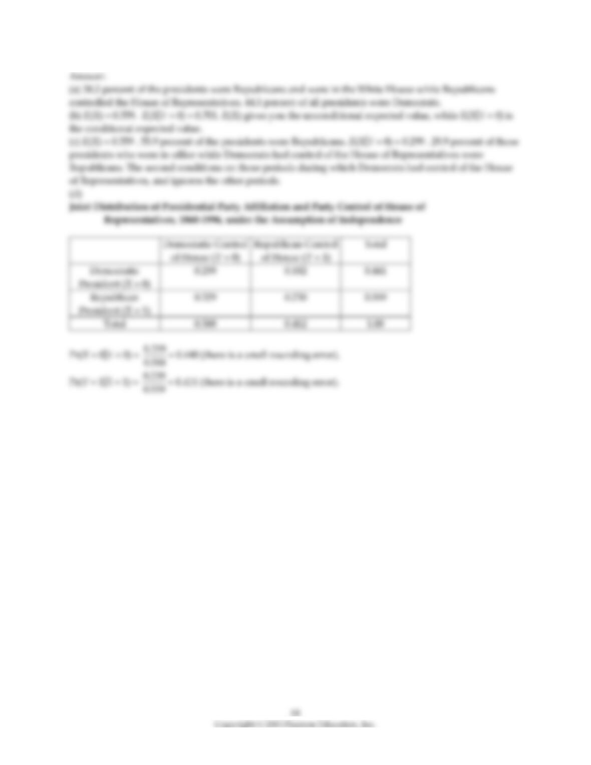
(d) What would the joint distribution look like under independence? Check your results by calculating
the two conditional distributions and compare these to the marginal distribution.