9) The expectations augmented Phillips curve postulates
△
p = π – f (u – ),
where
△
p is the actual inflation rate, π is the expected inflation rate, and u is the unemployment rate,
with “–” indicating equilibrium (the NAIRU – Non–Accelerating Inflation Rate of Unemployment). Under
the assumption of static expectations (π =
△
p–1), i.e., that you expect this period’s inflation rate to hold
for the next period (“the sun shines today, it will shine tomorrow”), then the prediction is that inflation
will accelerate if the unemployment rate is below its equilibrium level. The accompanying table below
displays information on accelerating annual inflation and unemployment rate differences from the
equilibrium rate (cyclical unemployment), where the latter is approximated by a five–year moving
average. You think of this data as a population which you want to describe, rather than a sample from
which you want to infer behavior of a larger population. The data is collected from United States
quarterly data for the period 1964:1 to 1995:4.
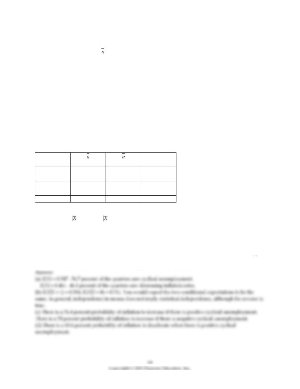
Joint Distribution of Accelerating Inflation and Cyclical Unemployment,
1964:1–1995:4
(u – ) > 0
(Y = 0)
(u – ) ≥ 0
(Y = 1)
Total
△
p–
△
p–1 > 0
(X = 0)
0.156
0.383
0.539
△
p–
△
p–1 ≤ 0
(X = 1)
0.297
0.164
0.461
Total
0.453
0.547
1.00
(a) Compute E(Y) and E(X), and interpret both numbers.
(b) Calculate E(Y= 1) and E(Y= 0). If there was independence between cyclical unemployment and
acceleration in the inflation rate, what would you expect the relationship between the two expected
values to be? Given that the two means are different, is this sufficient to assume that the two variables are
independent?
(c) What is the probability of inflation to increase if there is positive cyclical unemployment? Negative
cyclical unemployment?
(d) You randomly select one of the 59 quarters when there was positive cyclical unemployment ((u –
u
) >
0). What is the probability there was decelerating inflation during that quarter?
10) The accompanying table shows the joint distribution between the change of the unemployment rate in
an election year and the share of the candidate of the incumbent party since 1928. You think of this data
as a population which you want to describe, rather than a sample from which you want to infer behavior
of a larger population.
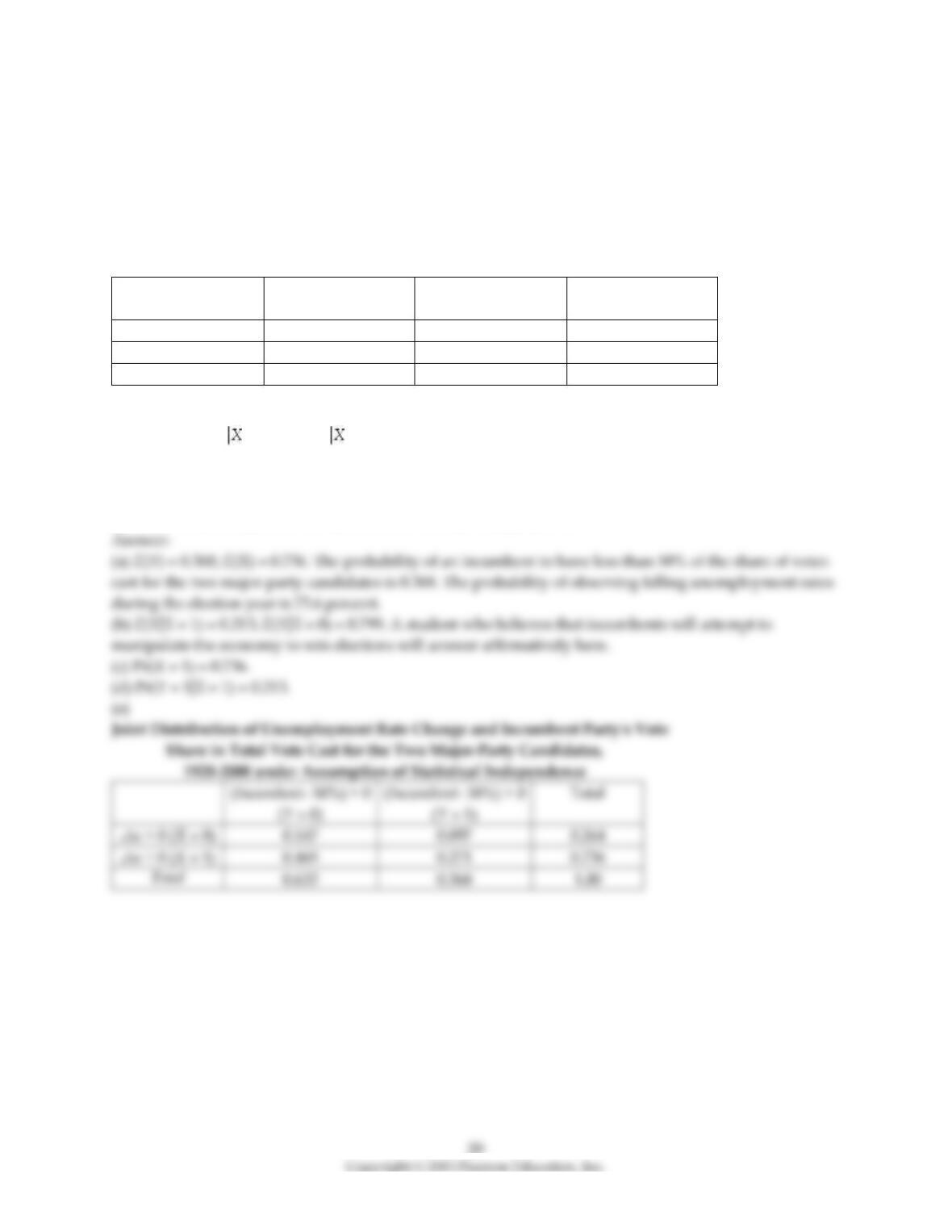
Joint Distribution of Unemployment Rate Change and Incumbent Party’s Vote
Share in Total Vote Cast for the Two Major–Party Candidates,
1928–2000
(Incumbent– 50%) > 0
(Y = 0)
(Incumbent– 50%) ≤ 0
(Y = 1)
Total
△
u > 0 (X = 0)
0.053
0.211
0.264
△
u ≤ 0 (X = 1)
0.579
0.157
0.736
Total
0.632
0.368
1.00
(a) Compute and interpret E(Y) and E(X).
(b) Calculate E(Y = 1) and E(Y = 0). Did you expect these to be very different?
(c) What is the probability that the unemployment rate decreases in an election year?
(d) Conditional on the unemployment rate decreasing, what is the probability that an incumbent will lose
the election?
(e) What would the joint distribution look like under independence?
(Incumbent– 50%) > 0
(Y = 0)
(Incumbent– 50%) > 0
(Y = 1)
0.167
0.097
0.465
0.271
0.632
0.368
11) The table accompanying lists the joint distribution of unemployment in the United States in 2001 by
demographic characteristics (race and gender).
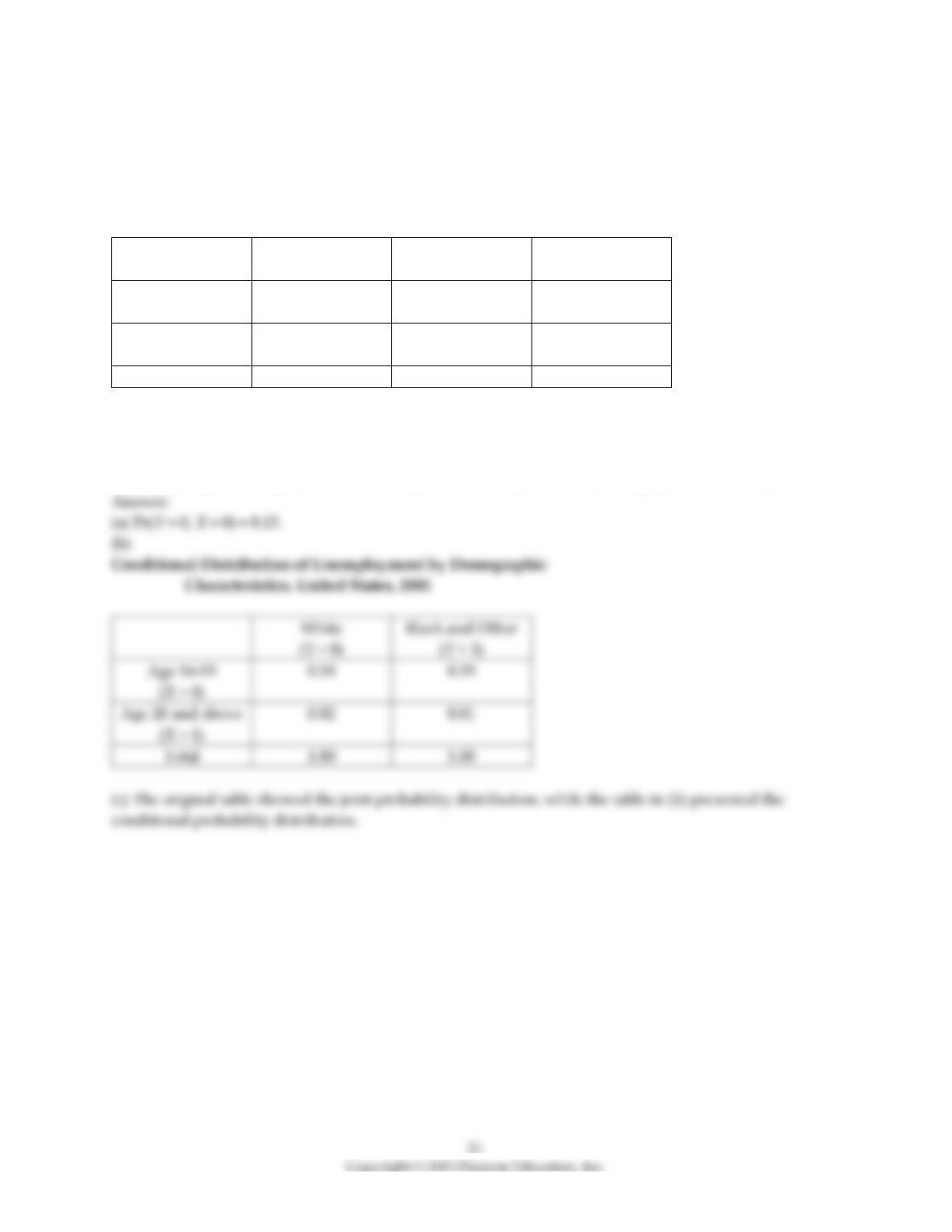
Joint Distribution of Unemployment by Demographic Characteristics,
United States, 2001
White
(Y = 0)
Black and Other
(Y = 1)
Total
Age 16-19
(X = 0)
0.13
0.05
0.18
Age 20 and above
(X = 1)
0.60
0.22
0.82
Total
0.73
0.27
1.00
(a) What is the percentage of unemployed white teenagers?
(b) Calculate the conditional distribution for the categories “white” and “black and other.”
(c) Given your answer in the previous question, how do you reconcile this fact with the probability to be
60% of finding an unemployed adult white person, and only 22% for the category “black and other.”
(Y = 0)
(Y = 1)
Age 16-19
(X = 0)
0.18
0.19
Age 20 and above
(X = 1)
0.82
0.81
Total
1.00
1.00
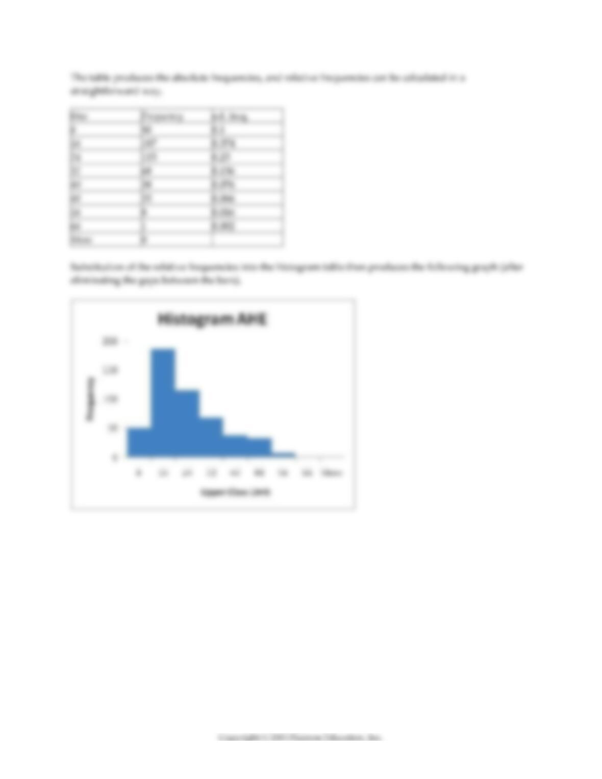
12) From the Stock and Watson (http://www.pearsonhighered.com/stock_watson) website the chapter 8
CPS data set (ch8_cps.xls) into a spreadsheet program such as Excel. For the exercise, use the first 500
observations only. Using data for average hourly earnings only (ahe), describe the earnings distribution.
Use summary statistics, such as the mean, median, variance, and skewness. Produce a frequency
distribution (“histogram”) using reasonable earnings class sizes.
23
2.3 Mathematical and Graphical Problems
1) Think of an example involving five possible quantitative outcomes of a discrete random variable and
attach a probability to each one of these outcomes. Display the outcomes, probability distribution, and
cumulative probability distribution in a table. Sketch both the probability distribution and the cumulative
probability distribution.
2) The height of male students at your college/university is normally distributed with a mean of 70 inches
and a standard deviation of 3.5 inches. If you had a list of telephone numbers for male students for the
purpose of conducting a survey, what would be the probability of randomly calling one of these students
whose height is
(a) taller than 6’0″?
(b) between 5’3″ and 6’5″?
(c) shorter than 5’7″, the mean height of female students?
(d) shorter than 5’0″?
(e) taller than Shaquille O’Neal, the center of the Boston Celtics, who is 7’1″ tall?
Compare this to the probability of a woman being pregnant for 10 months (300 days), where days of
pregnancy is normally distributed with a mean of 266 days and a standard deviation of 16 days.

3) Calculate the following probabilities using the standard normal distribution. Sketch the probability
distribution in each case, shading in the area of the calculated probability.
(a) Pr(Z < 0.0)
(b) Pr(Z ≤ 1.0)
(c) Pr(Z > 1.96)
(d) Pr(Z < –2.0)
(e) Pr(Z > 1.645)
(f) Pr(Z > –1.645)
(g) Pr(–1.96 < Z < 1.96)
(h.) Pr(Z < 2.576 or Z > 2.576)
(i.) Pr(Z > z) = 0.10; find z.
(j.) Pr(Z < –z or Z > z) = 0.05; find z.
4) Using the fact that the standardized variable Z is a linear transformation of the normally distributed
random variable Y, derive the expected value and variance of Z.
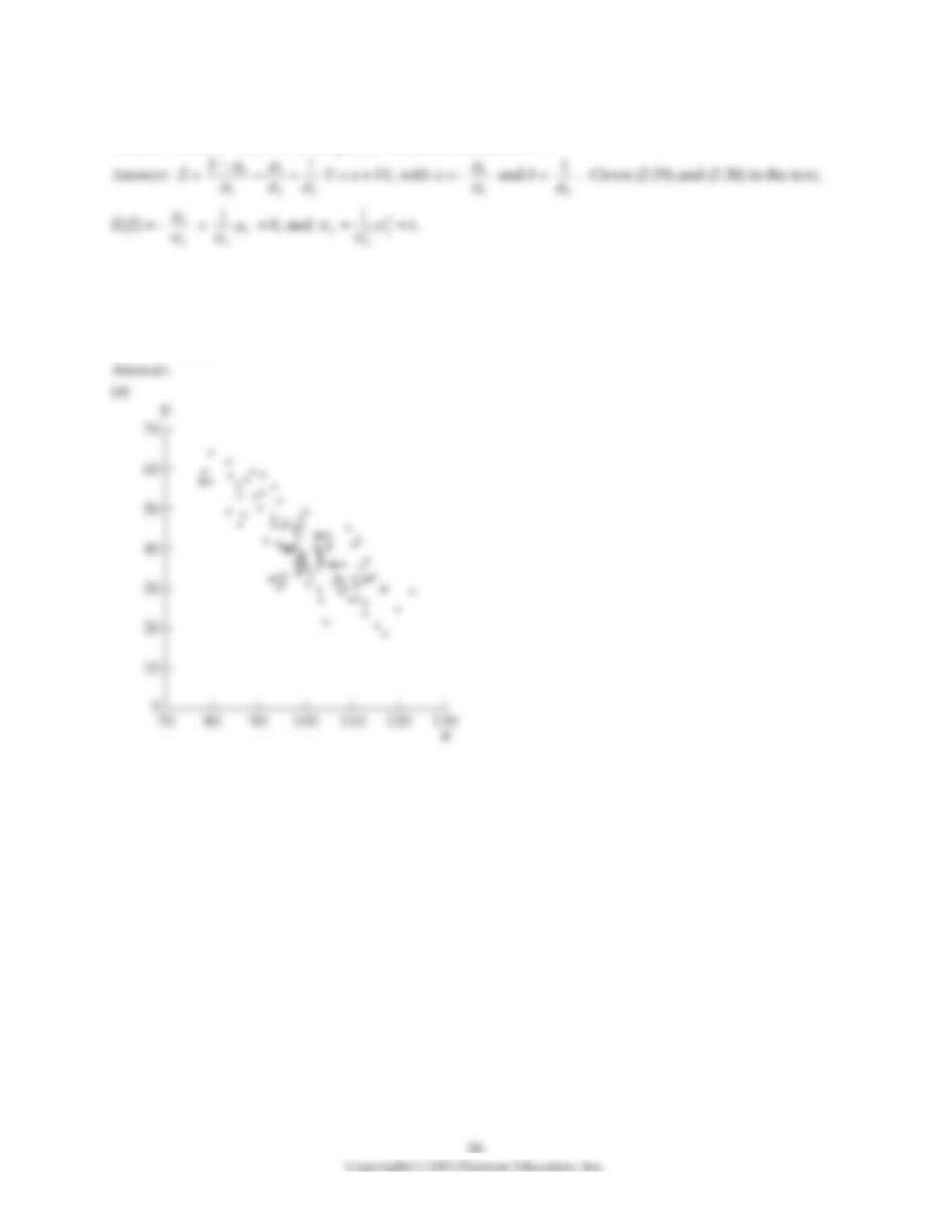
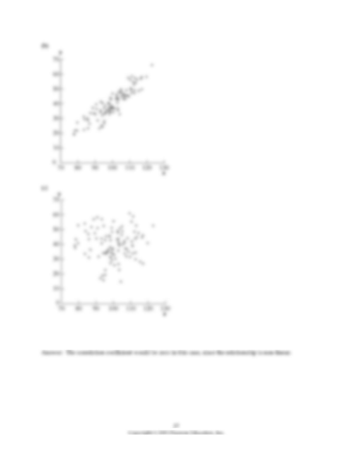
5) Show in a scatterplot what the relationship between two variables X and Y would look like if there was
(a) a strong negative correlation.
(b) a strong positive correlation.
(c) no correlation.
6) What would the correlation coefficient be if all observations for the two variables were on a curve
described by Y = X2?
7) Find the following probabilities:
(a) Y is distributed
2
4
X
. Find Pr(Y > 9.49).
(b) Y is distributed t∞. Find Pr(Y > –0.5).
(c) Y is distributed F4, ∞. Find Pr(Y < 3.32).
(d) Y is distributed N(500, 10000). Find Pr(Y > 696 or Y < 304).
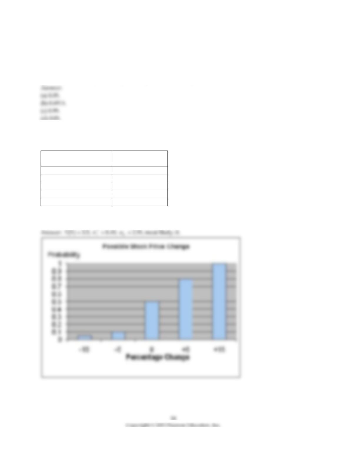
8) In considering the purchase of a certain stock, you attach the following probabilities to possible
changes in the stock price over the next year.
Stock Price Change During
Next Twelve Months (%)
Probability
+15
0.2
+5
0.3
0
0.4
–5
0.05
–15
0.05
What is the expected value, the variance, and the standard deviation? Which is the most likely outcome?
Sketch the cumulative distribution function.
9) You consider visiting Montreal during the break between terms in January. You go to the relevant Web
site of the official tourist office to figure out the type of clothes you should take on the trip. The site lists
that the average high during January is –7° C, with a standard deviation of 4° C. Unfortunately you are
more familiar with Fahrenheit than with Celsius, but find that the two are related by the following linear
function: C=
5
9
(F – 32).
Find the mean and standard deviation for the January temperature in Montreal in Fahrenheit.
10) Two random variables are independently distributed if their joint distribution is the product of their
marginal distributions. It is intuitively easier to understand that two random variables are independently
distributed if all conditional distributions of Y given X are equal. Derive one of the two conditions from
the other.
11) There are frequently situations where you have information on the conditional distribution of Y given
X, but are interested in the conditional distribution of X given Y. Recalling Pr(Y = y = x) =
Pr( , )
Pr( )
X x Y y
Xx
==
=
, derive a relationship between Pr(X = x = y) and Pr(Y = y = x). This is called Bayes’
theorem.
30
12) You are at a college of roughly 1,000 students and obtain data from the entire freshman class (250
students) on height and weight during orientation. You consider this to be a population that you want to
describe, rather than a sample from which you want to infer general relationships in a larger population.
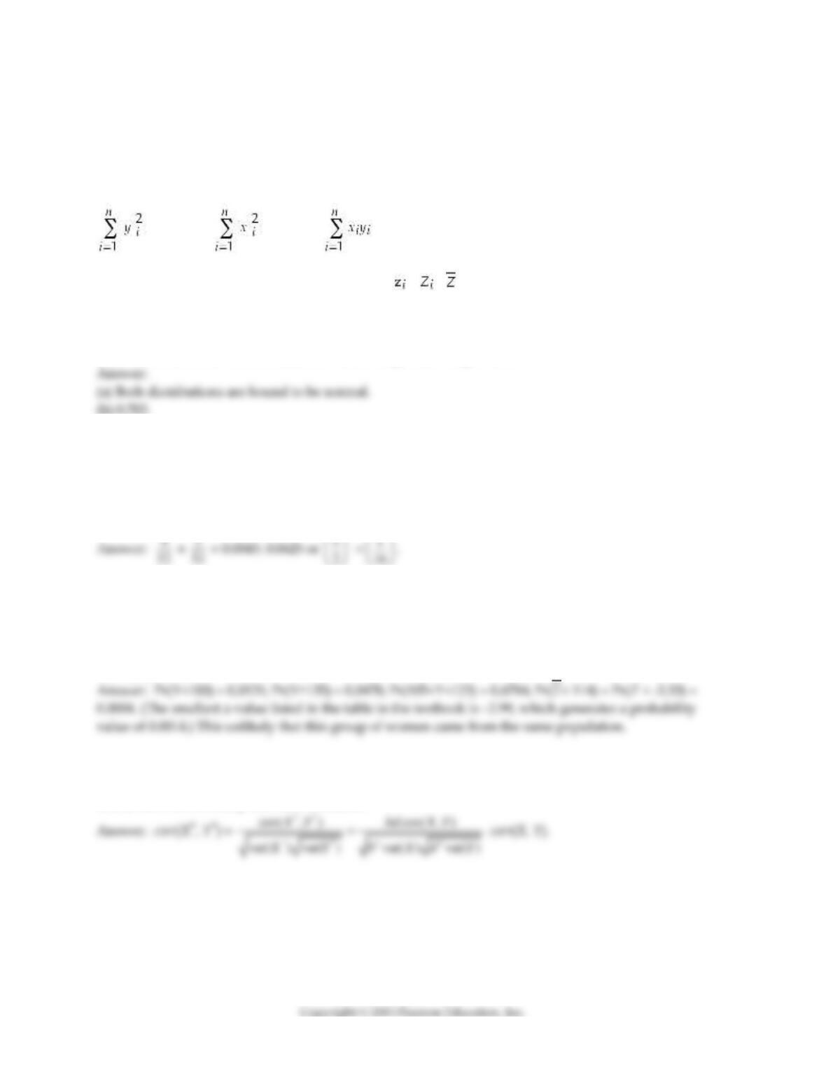
Weight (Y) is measured in pounds and height (X) is measured in inches. You calculate the following
sums:
= 94,228.8, = 1,248.9, = 7,625.9
(small letters refer to deviations from means as in = – ).
(a) Given your general knowledge about human height and weight of a given age, what can you say
about the shape of the two distributions?
(b) What is the correlation coefficient between height and weight here?
13) Use the definition for the conditional distribution of Y given X = x and the marginal distribution of X
to derive the formula for Pr(X = x, Y = y). This is called the multiplication rule. Use it to derive the
probability for drawing two aces randomly from a deck of cards (no joker), where you do not replace the
card after the first draw. Next, generalizing the multiplication rule and assuming independence, find the
probability of having four girls in a family with four children.
4
14) The systolic blood pressure of females in their 20s is normally distributed with a mean of 120 with a
standard deviation of 9. What is the probability of finding a female with a blood pressure of less than
100? More than 135? Between 105 and 123? You visit the women’s soccer team on campus, and find that
the average blood pressure of the 25 members is 114. Is it likely that this group of women came from the
same population?
15) Show that the correlation coefficient between Y and X is unaffected if you use a linear transformation
in both variables. That is, show that corr(X,Y) = corr(X*, Y*), where X* = a + bX and Y* = c + dY, and where
a, b, c, and d are arbitrary non–zero constants.
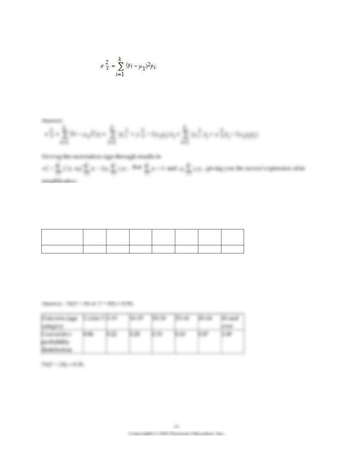
16) The textbook formula for the variance of the discrete random variable Y is given as
Another commonly used formulation is
2 2 2
1
k
Y i i Y
i
yp
=
=−
.
Prove that the two formulas are the same.
17) The Economic Report of the President gives the following age distribution of the United States
population for the year 2000:
United States Population By Age Group, 2000
Outcome (age
category
Under 5
5–15
16–19
20–24
25–44
45–64
65 and
over
Percentage
0.06
0.16
0.06
0.07
0.30
0.22
0.13
Imagine that every person was assigned a unique number between 1 and 275,372,000 (the total
population in 2000). If you generated a random number, what would be the probability that you had
drawn someone older than 65 or under 16? Treating the percentages as probabilities, write down the
cumulative probability distribution. What is the probability of drawing someone who is 24 years or
younger?
category
over
distribution
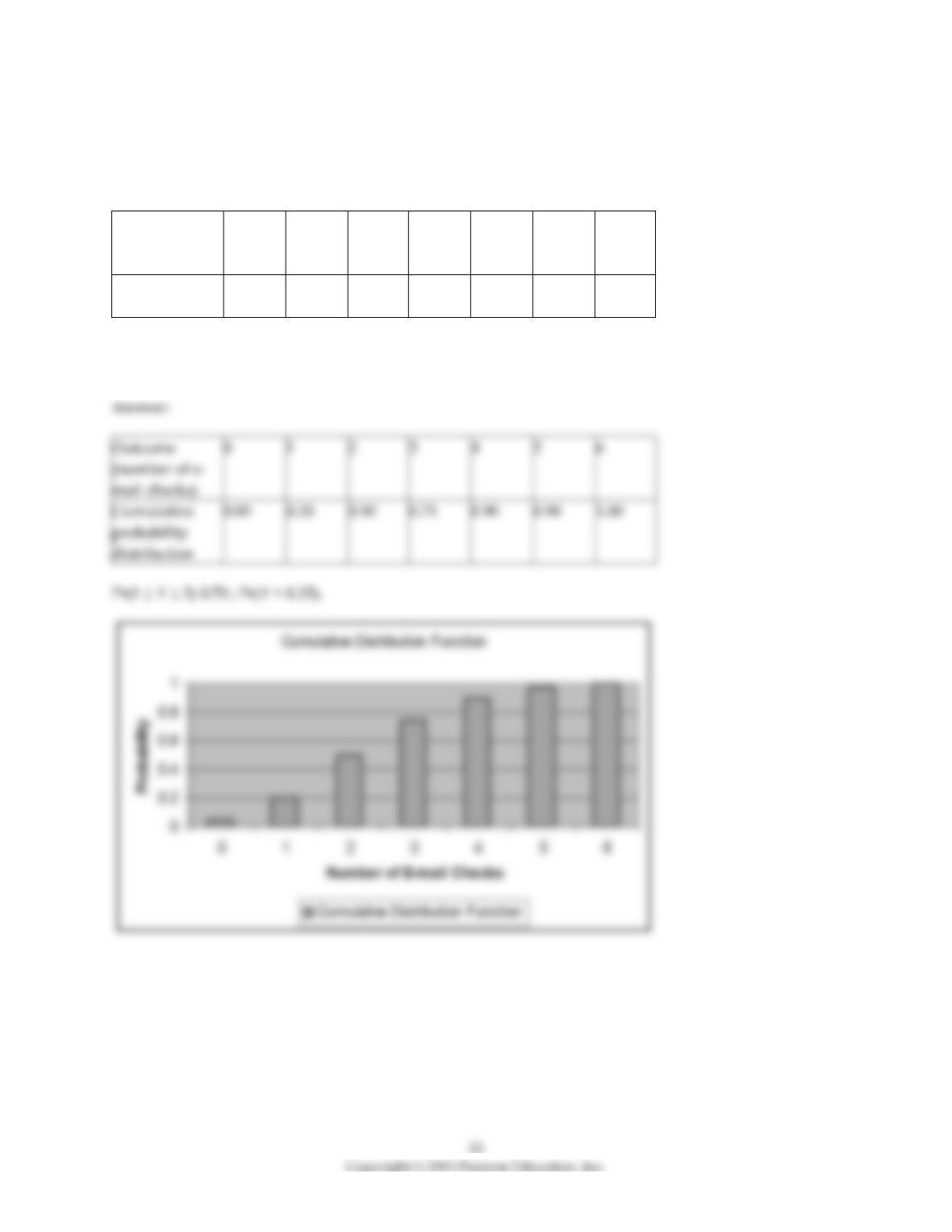
18) The accompanying table gives the outcomes and probability distribution of the number of times a
student checks her e–mail daily:
Probability of Checking E–Mail
Outcome
(number of e–
mail checks)
0
1
2
3
4
5
6
Probability
distribution
0.05
0.15
0.30
0.25
0.15
0.08
0.02
Sketch the probability distribution. Next, calculate the c.d.f. for the above table. What is the probability of
her checking her e–mail between 1 and 3 times a day? Of checking it more than 3 times a day?
(number of e–
mail checks)
Cumulative
probability
distribution
0.05
0.20
0.50
0.75
0.90
0.98
1.00
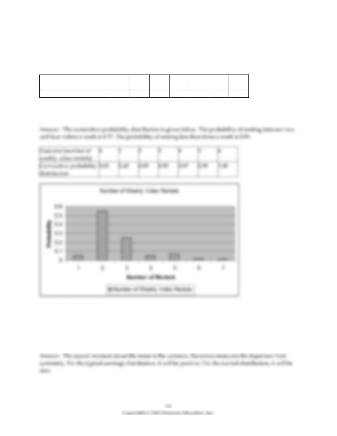
19) The accompanying table lists the outcomes and the cumulative probability distribution for a student
renting videos during the week while on campus.
Video Rentals per Week during Semester
Outcome (number of weekly
video rentals)
0
1
2
3
4
5
6
Probability distribution
0.05
0.55
0.25
0.05
0.07
0.02
0.01
Sketch the probability distribution. Next, calculate the cumulative probability distribution for the above
table. What is the probability of the student renting between 2 and 4 a week? Of less than 3 a week?
Outcome (number of
weekly video rentals)
0
1
2
3
4
5
6
Cumulative probability
distribution
0.05
0.60
0.85
0.90
0.97
0.99
1.00
20) The textbook mentioned that the mean of Y, E(Y) is called the first moment of Y, and that the expected
value of the square of Y, E(Y2) is called the second moment of Y, and so on. These are also referred to as
moments about the origin. A related concept is moments about the mean, which are defined as E[(Y –
µY)r]. What do you call the second moment about the mean? What do you think the third moment,
referred to as “skewness,” measures? Do you believe that it would be positive or negative for an earnings
distribution? What measure of the third moment around the mean do you get for a normal distribution?
21) Explain why the two probabilities are identical for the standard normal distribution:
Pr(–1.96 ≤ X ≤ 1.96) and Pr(–1.96 < X < 1.96).
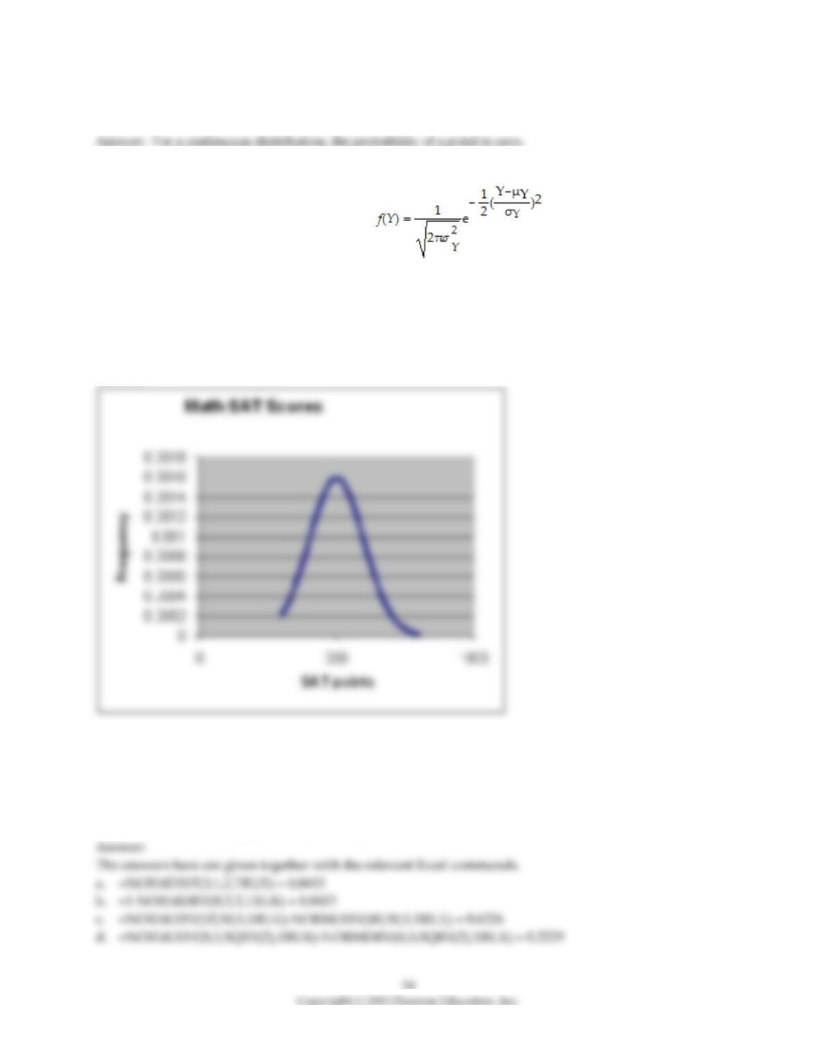
22) SAT scores in Mathematics are normally distributed with a mean of 500 and a standard deviation of
100. The formula for the normal distribution is . Use the scatter plot option
in a standard spreadsheet program, such as Excel, to plot the Mathematics SAT distribution using this
formula. Start by entering 300 as the first SAT score in the first column (the lowest score you can get in
the mathematics section as long as you fill in your name correctly), and then increment the scores by 10
until you reach 800. In the second column, use the formula for the normal distribution and calculate f(Y).
Then use the scatter plot option, where you eventually remove markers and substitute these with the
solid line option.
Answer:
23) Use a standard spreadsheet program, such as Excel, to find the following probabilities from various
distributions analyzed in the current chapter:
a. If Y is distributed N (1,4), find Pr(Y ≤ 3)
b. If Y is distributed N (3,9), find Pr(Y > 0)
c. If Y is distributed N (50,25), find Pr(40 ≤ Y ≤ 52)
d. If Y is distributed N (5,2), find Pr(6 ≤ Y ≤ 8)
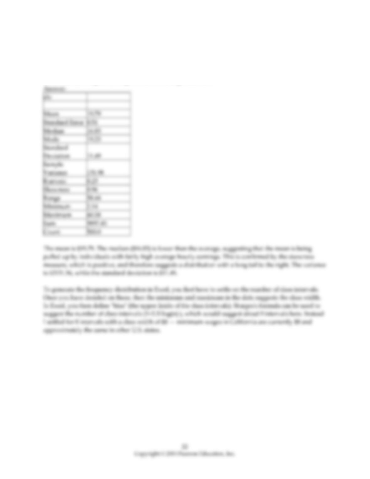
24) Looking at a large CPS data set with over 60,000 observations for the United States and the year 2004,
you find that the average number of years of education is approximately 13.6. However, a surprising
large number of individuals (approximately 800) have quite a low value for this variable, namely 6 years
or less. You decide to drop these observations, since none of your relatives or friends have that few years
of education. In addition, you are concerned that if these individuals cannot report the years of education
correctly, then the observations on other variables, such as average hourly earnings, can also not be
trusted. As a matter of fact you have found several of these to be below minimum wages in your state.
Discuss if dropping the observations is reasonable.
25) Use a standard spreadsheet program, such as Excel, to find the following probabilities from various
distributions analyzed in the current chapter:
a. If Y is distributed
2
4
X
, find Pr(Y ≤ 7.78)
b. If Y is distributed
2
10
X
, find Pr(Y > 18.31)
c. If Y is distributed F10,∞, find Pr(Y > 1.83)
d. If Y is distributed t15, find Pr(Y > 1.75)
e. If Y is distributed t90, find Pr(–1.99 ≤Y ≤ 1.99)
f. If Y is distributed N(0,1), find Pr(–1.99 ≤Y ≤ 1.99)
g. If Y is distributed F10,4, find Pr(Y > 4.12)
h. If Y is distributed F7,120, find Pr(Y > 2.79)