
Introduction to Econometrics, 3e (Stock)
Chapter 18 The Theory of Multiple Regression
18.1 Multiple Choice
1) The extended least squares assumptions in the multiple regression model include four assumptions
from Chapter 6 (ui has conditional mean zero; (Xi,Yi), i = 1,…, n are i.i.d. draws from their joint
distribution; Xi and ui have nonzero finite fourth moments; there is no perfect multicollinearity). In
addition, there are two further assumptions, one of which is
A) heteroskedasticity of the error term.
B) serial correlation of the error term.
C) homoskedasticity of the error term.
D) invertibility of the matrix of regressors.
2) The difference between the central limit theorems for a scalar and vector–valued random variables is
A) that n approaches infinity in the central limit theorem for scalars only.
B) the conditions on the variances.
C) that single random variables can have an expected value but vectors cannot.
D) the homoskedasticity assumption in the former but not the latter.
3) The Gauss–Markov theorem for multiple regression states that the OLS estimator
A) has the smallest variance possible for any linear estimator.
B) is BLUE if the Gauss–Markov conditions for multiple regression hold.
C) is identical to the maximum likelihood estimator.
D) is the most commonly used estimator.
4) The GLS assumptions include all of the following, with the exception of
A) the Xi are fixed in repeated samples.
B) Xi and ui have nonzero finite fourth moments.
C) E(U) = Ω(X), where Ω(X) is n × n matrix–valued that can depend on X.
D) E(U) = 0n.
5) The multiple regression model can be written in matrix form as follows:
A) Y = Xβ.
B) Y = X + U.
C) Y = βX + U.
D) Y = Xβ + U.

6) The linear multiple regression model can be represented in matrix notation as Y= Xβ + U, where X is of
order n×(k+1). k represents the number of
A) regressors.
B) observations.
C) regressors excluding the “constant” regressor for the intercept.
D) unknown regression coefficients.
7) The multiple regression model in matrix form Y = Xβ + U can also be written as
A) Yi = β0 + Xβ + ui, i = 1,…, n.
B) Yi = Xβi, i = 1,…, n.
C) Yi = βX + ui, i = 1,…, n.
D) Yi = Xβ + ui, i = 1,…, n.
8) The assumption that X has full column rank implies that
A) the number of observations equals the number of regressors.
B) binary variables are absent from the list of regressors.
C) there is no perfect multicollinearity.
D) none of the regressors appear in natural logarithm form.
9) One implication of the extended least squares assumptions in the multiple regression model is that
A) feasible GLS should be used for estimation.
B) E(U|X) = In.
C) X is singular.
D) the conditional distribution of U given X is N(0n, In).
10) One of the properties of the OLS estimator is
A) X= 0k+1.
B) that the coefficient vector has full rank.
C) (Y – X ) = 0k+1.
D) ( X)–1= Y
11) Minimization of results in
A) Y = X.
B) X = 0k+1.
C) (Y – X) = 0k+1.
D) Rβ = r.
12) The Gauss–Markov theorem for multiple regression proves that
A) MX is an idempotent matrix.
B) the OLS estimator is BLUE.
C) the OLS residuals and predicted values are orthogonal.
D) the variance–covariance matrix of the OLS estimator is (X)–1.
13) The GLS estimator is defined as
A) ( Ω–1X)–1 ( Ω–1Y).
B) ( X)–1Y.
C) Y.
D) ( X)–1U.
14) The OLS estimator
A) has the multivariate normal asymptotic distribution in large samples.
B) is t–distributed.
C) has the multivariate normal distribution regardless of the sample size.
D) is F–distributed.
15) – β
A) cannot be calculated since the population parameter is unknown.
B) = ( X)–1U.
C) = Y – .
D) = β + ( X)–1U

16) The heteroskedasticity–robust estimator of
( )
ˆ
n
−
is obtained
A) from ( X)–1U.
B) by replacing the population moments in its definition by the identity matrix.
C) from feasible GLS estimation.
D) by replacing the population moments in its definition by sample moments.
17) A joint hypothesis that is linear in the coefficients and imposes a number of restrictions can be written
as
A) ( X)–1Y.
B) Rβ = r.
C) – β.
D) Rβ= 0.
18) Let there be q joint hypothesis to be tested. Then the dimension of r in the expression
Rβ = r is
A) q × 1.
B) q × (k+1).
C) (k+1) × 1.
D) q.
19) The formulation Rβ= r to test a hypotheses
A) allows for restrictions involving both multiple regression coefficients and single regression
coefficients.
B) is F–distributed in large samples.
C) allows only for restrictions involving multiple regression coefficients.
D) allows for testing linear as well as nonlinear hypotheses.
20) Let PX = X( X)–1 and MX = In – PX. Then MX MX =
A) X( X)–1 – PX.
B)
C) In.
D) MX.
21) In the case when the errors are homoskedastic and normally distributed, conditional on X, then
A) is distributed N(β, ),where = I(k+1).
B) is distributed N(β, ), where = /n = /n.
C) is distributed N(β, ),where = ( X)–1.
D) = PXY where PX = X(X)–1.
22) An estimator of β is said to be linear if
A) it can be estimated by least squares.
B) it is a linear function of Y1,…, Yn .
C) there are homoskedasticity–only errors.
D) it is a linear function of X1,…, Xn .
23) The leading example of sampling schemes in econometrics that do not result in independent
observations is
A) cross–sectional data.
B) experimental data.
C) the Current Population Survey.
D) when the data are sampled over time for the same entity.
24) The presence of correlated error terms creates problems for inference based on OLS. These can be
overcome by
A) using HAC standard errors.
B) using heteroskedasticity–robust standard errors.
C) reordering the observations until the correlation disappears.
D) using homoskedasticity–only standard errors.
25) The GLS estimator
A) is always the more efficient estimator when compared to OLS.
B) is the OLS estimator of the coefficients in a transformed model, where the errors of the transformed
model satisfy the Gauss–Markov conditions.
C) cannot handle binary variables, since some of the transformations require division by one of the
regressors.
D) produces identical estimates for the coefficients, but different standard errors.
26) The extended least squares assumptions in the multiple regression model include four assumptions
from Chapter 6 (ui has conditional mean zero; (Xi,Yi), i = 1,…, n are i.i.d. draws from their joint
distribution; Xi and ui have nonzero finite fourth moments; there is no perfect multicollinearity). In
addition, there are two further assumptions, one of which is
A) heteroskedasticity of the error term.
B) serial correlation of the error term.
C) the conditional distribution of ui given Xi is normal.
D) invertibility of the matrix of regressors.
27) The OLS estimator for the multiple regression model in matrix form is
A) (X’X)–1X’Y
B) X(X’X)–1X’ – PX
C) (X’X)–1X’U
D) (XΩ–1X)–1XΩ–1Y
28) To prove that the OLS estimator is BLUE requires the following assumption
A) (Xi,Yi) i = 1, …, n are i.i.d. draws from their joint distribution
B) Xi and ui have nonzero finite fourth moments
C) the conditional distribution of ui given Xi is normal
D) none of the above
29) The TSLS estimator is
A) (X’X)–1 X’Y
B) (X’Z(Z’Z)–1 Z’X)–1 X’Z(Z’Z)–1 Z’ Y
C) (XΩ–1X)–1(XΩ–1Y)
D) (X’Pz)–1PzY
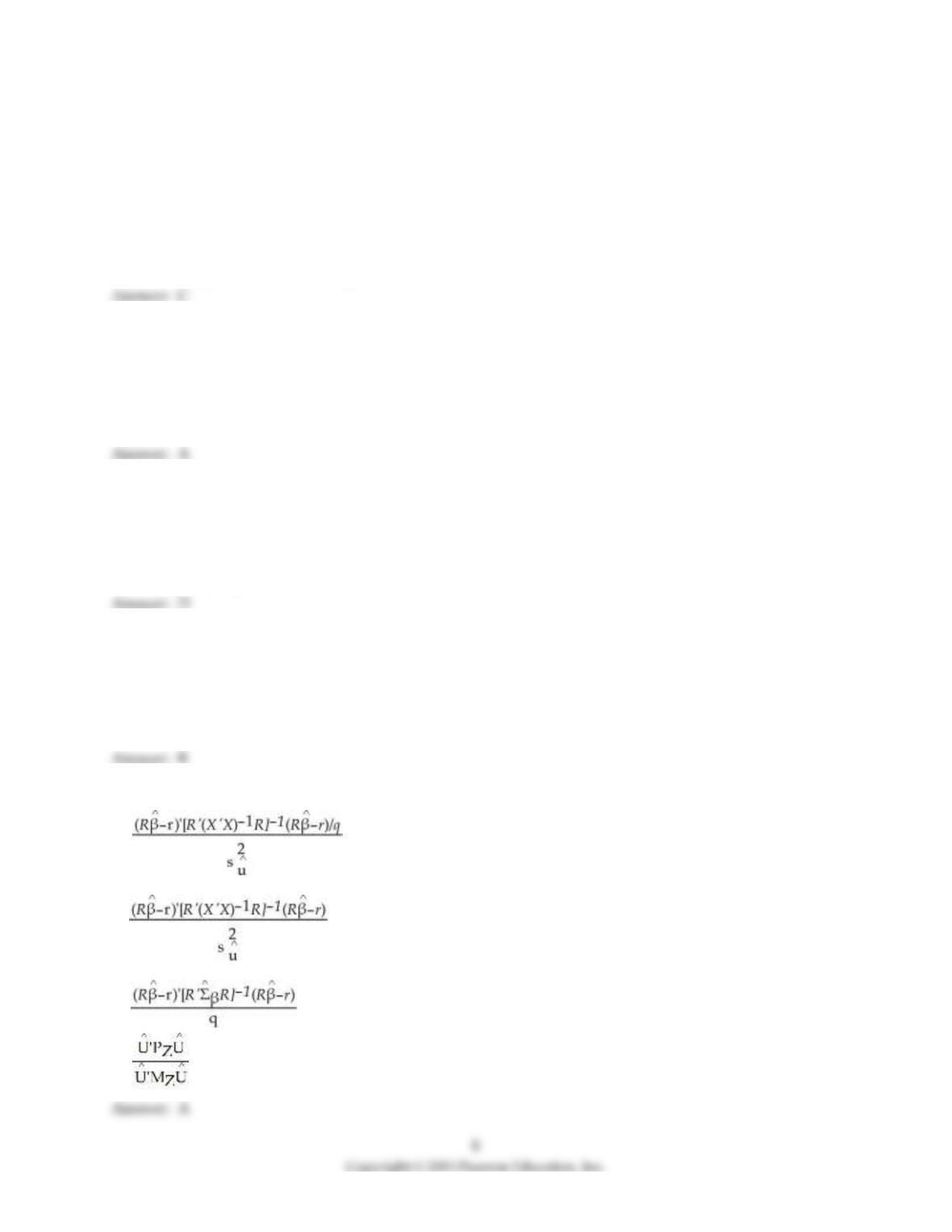
30) The homoskedasticity–only F–statistic is
A)
B)
C)
D)
18.2 Essays and Longer Questions
1) Write an essay on the difference between the OLS estimator and the GLS estimator.
2) Give several economic examples of how to test various joint linear hypotheses using matrix notation.
Include specifications of Rβ = r where you test for (i) all coefficients other than the constant being zero,
(ii) a subset of coefficients being zero, and (iii) equality of coefficients. Talk about the possible
distributions involved in finding critical values for your hypotheses.
3) Define the GLS estimator and discuss its properties when Ω is known. Why is this estimator sometimes
called infeasible GLS? What happens when Ω is unknown? What would the Ω matrix look like for the
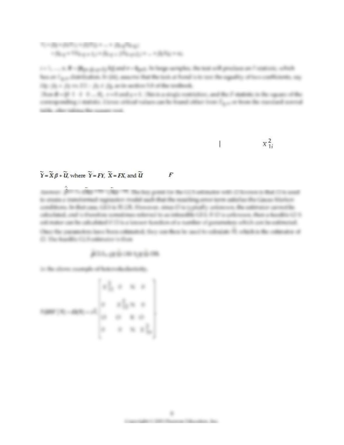
case of independent sampling with heteroskedastic errors, where var(ui Xi) = ch(Xi) = σ2? Since the
inverse of the error variance–covariance matrix is needed to compute the GLS estimator, find Ω–1. The
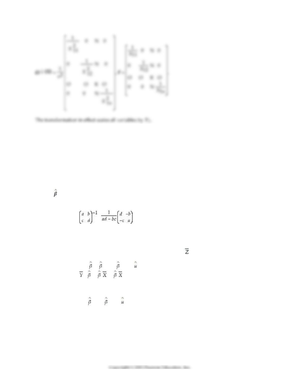
textbook shows that the original model Y = Xβ + U will be transformed into
= FU, and F = Ω–1. Find F in the above case, and describe what
effect the transformation has on the original data.
10
4) Consider the multiple regression model from Chapter 5, where k = 2 and the assumptions of the
multiple regression model hold.
(a) Show what the X matrix and the β vector would look like in this case.
(b) Having collected data for 104 countries of the world from the Penn World Tables, you want to
estimate the effect of the population growth rate (X1i) and the saving rate (X2i) (average investment share
of GDP from 1980 to 1990) on GDP per worker (relative to the U.S.) in 1990. What are your expected signs
for the regression coefficient? What is the order of the (X’X) here?
(c) You are asked to find the OLS estimator for the intercept and slope in this model using the
formula = (X’X)–1 X’Y. Since you are more comfortable in inverting a 2×2 matrix (the inverse of a 2×2
matrix is,
= )
you decide to write the multiple regression model in deviations from mean form. Show what the X
matrix, the (X’X) matrix, and the X’Y matrix would look like now.
(Hint: use small letters to indicate deviations from mean, i.e., zi = Zi – and note that
Yi = 0 + 1X1i + 2X2i + i
= 0 + 1 1 + 2 2.
Subtracting the second equation from the first, you get
yi = 1x1i + 2x2i + i)
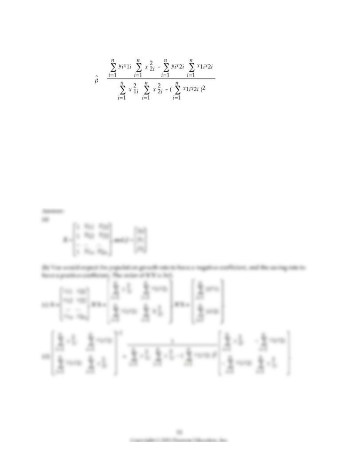
(d) Show that the slope for the population growth rate is given by
1 =
(e) The various sums needed to calculate the OLS estimates are given below:
2
1
n
i
i
y
=
= 8.3103;
2
1
1
n
i
i
x
=
= .0122;
2
2
1
n
i
i
x
=
= 0.6422
1
1
n
ii
i
yx
=
= –0.2304;
2
1
n
ii
i
yx
=
= 1.5676;
12
1
n
ii
i
xx
=
= –0.0520
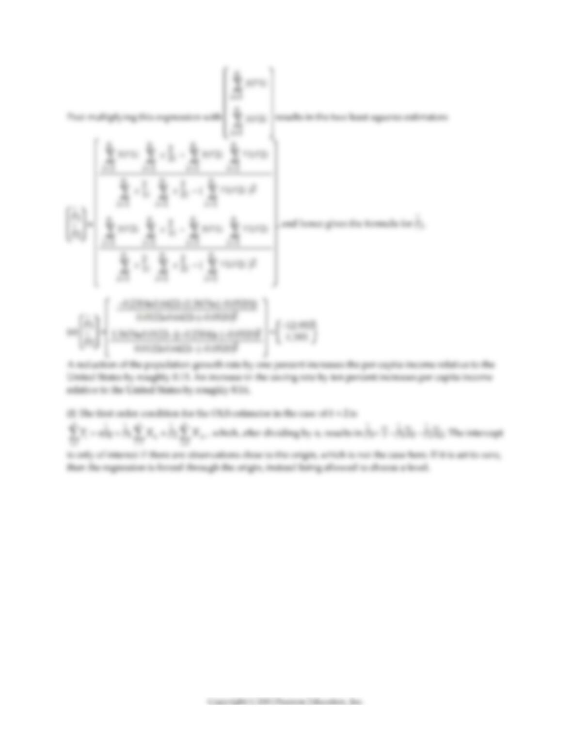
Find the numerical values for the effect of population growth and the saving rate on per capita income
and interpret these.
(f) Indicate how you would find the intercept in the above case. Is this coefficient of interest in the
interpretation of the determinants of per capita income? If not, then why estimate it?
12