3) Purchasing power parity (PPP), postulates that the exchange rate between two countries equals the
ratio of the respective price indexes or ExchRate = (where ExchRate is the foreign exchange rate
between the two countries, and P represents the price index, with f indicating the foreign country). The
long–run version of PPP implies that that the exchange rate and the price ratio share a common trend.
(a) You collect monthly foreign exchange rate data from 1974:1 to 2002:4 for the U.S./U.K. exchange rate
($/£) and you collect data on the Consumer Price Index for both countries. Explain how you would used
the Engle–Granger test statistic to investigate the long–run PPP hypothesis.
(b) One of your peers explains that there may be an easier way to test for the validity of PPP. She
suggests to simply test whether or not the “real” exchange rate, or competitiveness, is stationary. (The
real exchange rate is given by ExchRate × ) Is she correct? Explain. How would you implement her
suggestion? Which alternative test–statistic is available?
4) You have collected quarterly Canadian data on the unemployment and the inflation rate from 1962:I to
2001:IV. You want to re–estimate the ADL(3,1) formulation of the Phillips curve using a GARCH(1,1)
specification. The results are as follows:
t = 1.17 – .56 ΔInft–1 – .47 ΔInft–2 – .31 ΔInft–3 – .13 Unempt–1
(.48) (.08) (.10) (.09) (.06)
= .86 + .27 + .53 .
(.40) (.11) (.15)
(a) Test the two coefficients for and in the GARCH model individually for statistical
significance.
(b) Estimating the same equation by OLS results in
t = 1.19 – .51 ΔInft–1 – .47 ΔInft–2 – .28 ΔInft–3 – .16Unempt–1
(.54) (.10) (.11) (.08) (.07)
Briefly compare the estimates. Which of the two methods do you prefer?
(c) Given your results from the test in (a), what can you say about the variance of the error terms in the
Phillips Curve for Canada?
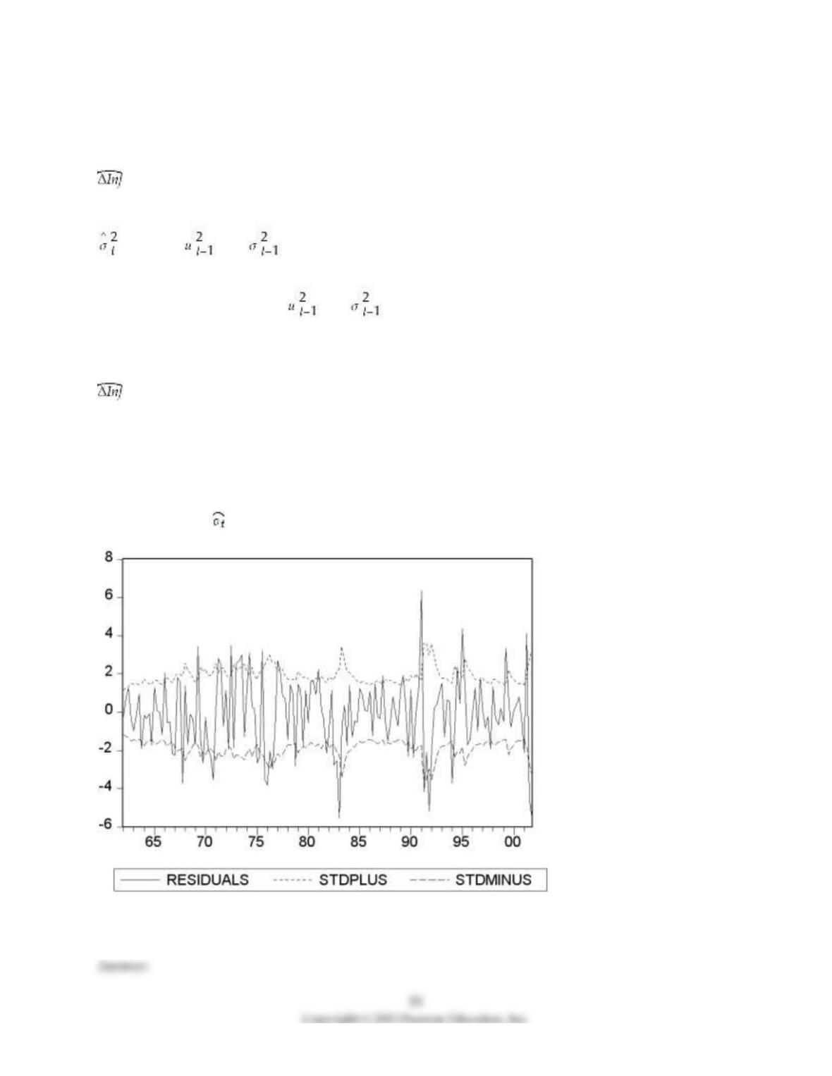
(d) The following figure plots the residuals along with bands of plus or minus one predicted standard
deviation (that is, ±) based on the GARCH(1,1) model.
Describe what you see.

17
6) Your textbook states that there “are three ways to decide if two variables can plausibly be modeled as
cointegrated: use expert knowledge and economic theory, graph the series and see whether they appear
to have a common stochastic trend, and perform statistical tests for cointegration. All three ways should
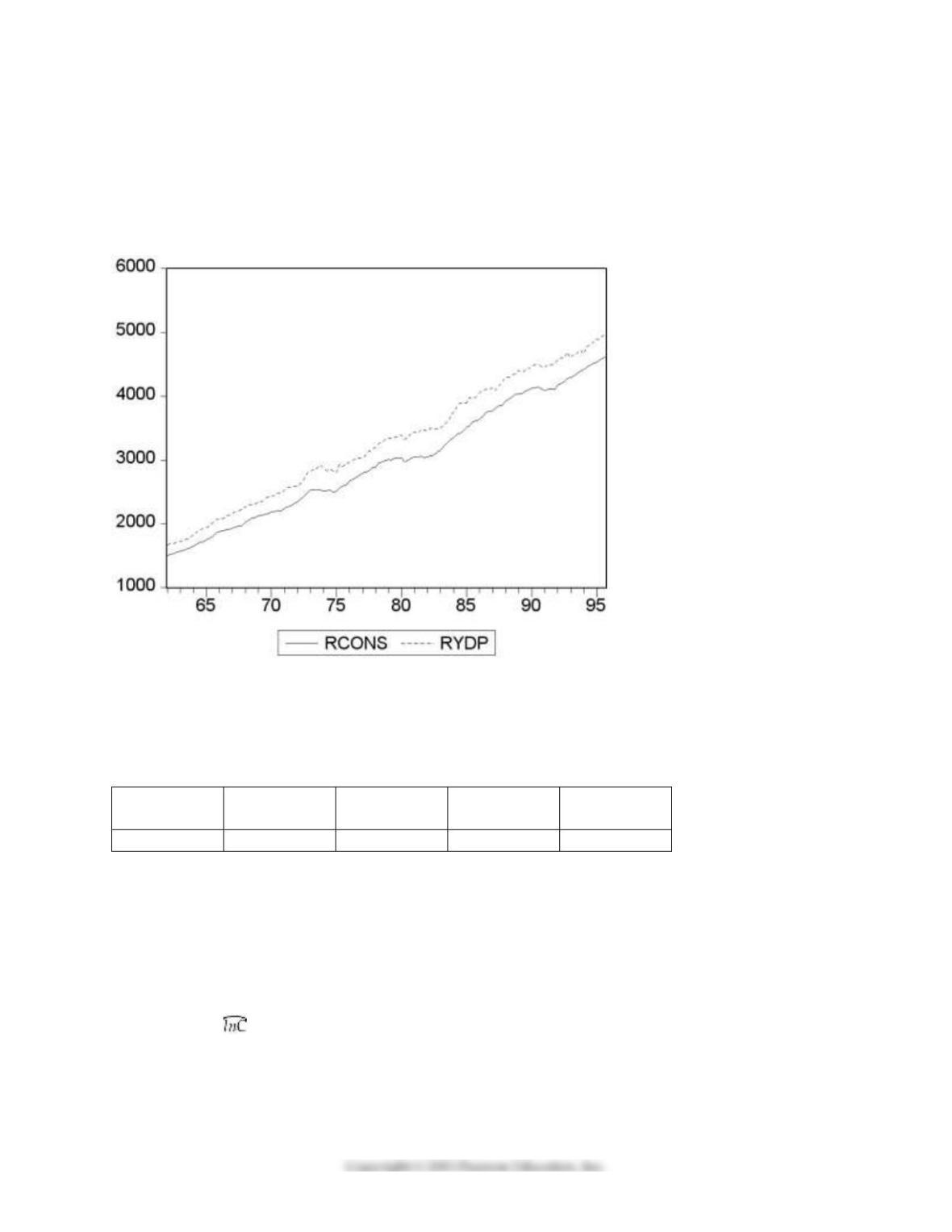
be used in practice.” Accordingly you set out to check whether (the log of) consumption and (the log of)
personal disposable income are cointegrated. You collect data for the sample period 1962:I to 1995:IV and
plot the two variables.
(a) Using the first two methods to examine the series for cointegration, what do you think the likely
answer is?
(b) You begin your numerical analysis by testing for a stochastic trend in the variables, using an
Augmented Dickey–Fuller test. The t–statistic for the coefficient of interest is as follows:
Variable with
lag of 1
LnYpd
ΔLnYpd
LnC
ΔLnC
t–statistic
–1.93
–5.24
–2.20
–4.31
where LnYpd is (the log of) personal disposable income, and LnC is (the log of) real consumption. The
estimated equation included an intercept for the two growth rates, and, in addition, a deterministic trend
for the level variables. For each case make a decision about the stationarity of the variables based on the
critical value of the Augmented Dickey–Fuller test statistic. Why do you think a trend was included for
level variables?
(c) Using the first step of the EG–ADF procedure, you get the following result:
t = -0.24 + 1.017 lnYpdt
Should you interpret this equation? Would you be impressed if you were told that the regression R2 was
0.998 and that the t–statistic for the slope was 266.06? Why or why not?
(d) The Dickey–Fuller test for the residuals for the cointegrating regressions results in a t–statistic of
(-3.64). State the null and alternative hypothesis and make a decision based on the result.
(e) You want to investigate if the slope of the cointegrating vector is one. To do so, you use the DOLS
estimator and HAC standard errors. The slope coefficient is 1.024 with a standard error of 0.009. Can you
reject the null hypothesis that the slope equals one?
7) Your textbook so far considered variables for cointegration that are integrated of the same order. For
example, the log of consumption and personal disposable income might both be I(1) variables, and the
error correction term would be I(0), if consumption and personal disposable income were cointegrated.
(a) Do you think that it makes sense to test for cointegration between two variables if they are integrated
of different orders? Explain.
(b) Would your answer change if you have three variables, two of which are I(1) while the third is I(0)?
Can you think of an example in this case?
8) For the United States, there is somewhat conflicting evidence whether or not the inflation rate has a
unit autoregressive root. For example, for the sample period 1962:I to 1999:IV using the ADF statistic,
you cannot reject at the 5% significance level that inflation contains a stochastic trend. However the null
hypothesis can be rejected at the 10% significance level. The DF–GLS test rejects the null hypothesis at the
five percent level. This result turns out to be sensitive to the number of lags chosen and the sample
period.
(a) Somewhat intrigued by these findings, you decide to repeat the exercise using Canadian data. Letting
the AIC choose the lag length of the ADF regression, which turns out to be three, the ADF statistic is
(–1.91). What is your decision regarding the null hypothesis?
(b) You also calculate the DF–GLS statistic, which turns out to be (–1.23). Can you reject the null
hypothesis in this case?
(c) Is it possible for the two test statistics to yield different answers and if so, why?
9) You have collected time series for various macroeconomic variables to test if there is a single
cointegrating relationship among multiple variables. Formulate the null hypothesis and compare the EG–
ADF statistic to its critical value.
(a) Canadian unemployment rate, Canadian Inflation Rate, United States unemployment rate, United
States inflation rate; t = (–3.374).
(b) Approval of United States presidents (Gallup poll), cyclical unemployment rate, inflation rate,
Michigan Index of Consumer Sentiment; t = (–3.837).
(c) The log of real GDP, log of real government expenditures, log of real money supply (M2); t = (–2.23).
(d) Briefly explain how you could potentially improve on VAR(p) forecasts by using a cointegrating
vector.
10) There has been much talk recently about the convergence of inflation rates between many of the
OECD economies. You want to see if there is evidence of this closer to home by checking whether or not
Canada’s inflation rate and the United States’ inflation rate are cointegrated.
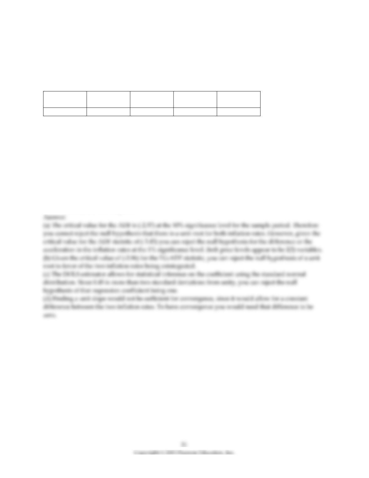
(a) You begin your numerical analysis by testing for a stochastic trend in the variables, using an
Augmented Dickey–Fuller test. The t–statistic for the coefficient of interest is as follows:
Variable with
lag of 1
InfCan
ΔInfCan
InfUS
ΔInfUS
t–statistic
–1.93
–6.38
–2.37
–5.63
where InfCan is the Canadian inflation rate, and InfUS is the United States inflation rate. The estimated
equation included an intercept. For each case make a decision about the stationarity of the variables based
on the critical value of the Augmented Dickey–Fuller test statistic.
(b) Your test for cointegration results in a EG–ADF statistic of (–7.34). Can you reject the null hypothesis
of a unit root for the residuals from the cointegrating regression?
(c) Using a working hypothesis that the two inflation rates are cointegrated, you want to test whether or
not the slope coefficient equals one. To do so you estimate the cointegrating equation using the DOLS
estimator with HAC standard errors. The coefficient on the U.S. inflation rate has a value of 0.45 with a
standard error of 0.13. Can you reject the null hypothesis that the slope equals unity?
(d) Even if you could not reject the null hypothesis of a unit slope, would that have been sufficient
evidence to establish convergence?
11) You have re–estimated the two variable VAR model of the change in the inflation rate and the
unemployment rate presented in your textbook using the sample period 1982:I (first quarter) to 2009:IV.
To see if the conclusions regarding Granger causality of changed, you conduct an F–test for this new
sample period. The results are as follows: The F–statistic testing the null hypothesis that the coefficients
on Unempt–1, Unempt–2, Unempt–3, and Unemplt–4 are zero in the inflation equation (Equation 16.5 in your
textbook) is 6.04. The F–statistic testing the hypothesis that the coefficients on the four lags of ΔInft are
zero in the unemployment equation (Equation 16.6 in your textbook) is 0.80.
a. What is the critical value of the F–statistic in both cases?
b. Do you think that the unemployment rate Granger–causes changes in the inflation rate?
c. Do you think that the change in the inflation rate Granger–causes the unemployment rate?
12) In this case, the Granger causality statistic does not exceed the critical value, and hence the conclusion
is that the change in the inflation rate does not Granger–cause the unemployment rate.
t = 0.05 – 0.31 ΔInft–1
(0.14) (0.07)
t = 1982:I – 2009:IV, R2 = 0.10, SER = 2.4
a. Calculate the one–quarter–ahead forecast of both ΔInf2010:I and Inf2010:I (the inflation rate in 2009:IV
was 2.6 percent, and the change in the inflation rate for that quarter was –1.04).
b. Calculate the forecast for 2010:II using the iterated multiperiod AR forecast both for the change in the
inflation rate and the inflation rate.
c. What alternative method could you have used to forecast two quarters ahead? Write down the
equation for the two–period ahead forecast, using parameters instead of numerical coefficients, which you
would have used.
13) You have collected quarterly data for real GDP (Y) for the United States for the period 1962:I (first
quarter) to 2009:IV.
a. Testing the log of GDP for stationarity, you run the following regression (where the lag length was
determined using the AIC):
t = 0.03 – 0.0024 lnYt–1 + 0.253 ΔlnYt–1 + 0.167 ΔlnYt–2
(0.03) (0.0014) (0.072) (0.072)
t = 1962:I – 2009:IV, R2 = 0.16, SER = 0.008
Use the ADF statistic with an intercept only to test for stationarity. What is your decision?
b. You have decided to test the growth rate of real GDP for stationarity for the same sample period. The
regression is as follows:
t = 0.0041 – 0.543 ΔlnYt–1 – 0.186 Δ2lnYt–1
(0.0009) (0.082) (0.071)
t = 1962:I – 2009:IV, R2 = 0.16, SER = 0.008
Use the ADF statistic with an intercept only to test for stationarity. What is your decision?
c. Using the orders of integration terminology, what order of integration is the log level of real GDP?
The growth rate?
d. Given that the SER hardly changed in the second equation, why is the regression R2 larger?
14) Economic theory suggests that the law of one price holds. Applying this concept to foreign and
domestic goods implies that goods will sell for the same price across countries. The consumer price index
is the price for a basket of goods, and is calculated for countries as a whole. Hence in the absence of
barriers to trade, and large transportation costs (and the fact that not all goods are traded) you should
observe Purchasing Power Parity (PPP) between two countries, or ExchRate × P = Pf, where ExchRate is
the foreign exchange rate between the two countries, and P represents the price index, with f indicating
the foreign country. Dividing both sides of the equation by the domestic price level then gives you the
standard formulation for PPP: ExchRate = . If PPP holds in the long run, then the exchange rate and
the price ratio should share a common trend. Since it is a long–run concept, cointegration provides an
interesting way to test for it.
a. Using monthly data for the U.S./U.K. exchange rate ($/₤) and the respective price indexes, you
estimate the following regression:
t = 0.44 + 0.69 (lnPUS – lnPUK)
Collecting the residuals from this regression and using an ADF test for cointegration, you find a t–statistic
of –2.71. Can you reject the null–hypothesis of no cointegration? What is the critical value?
b. Was it good econometric practice to test for cointegration right away? What else should you have
done before proceeding with the EG–ADF test?