20

7) Statistical inference was a concept that was not too difficult to understand when using cross–sectional
data. For example, it is obvious that a population mean is not the same as a sample mean (take weight of
students at your college/university as an example). With a bit of thought, it also became clear that the
sample mean had a distribution. This meant that there was uncertainty regarding the population mean
given the sample information, and that you had to consider confidence intervals when making statements
about the population mean. The same concept carried over into the two–dimensional analysis of a simple
regression: knowing the height–weight relationship for a sample of students, for example, allowed you to
make statements about the population height–weight relationship. In other words, it was easy to
understand the relationship between a sample and a population in cross–sections. But what about time–
series? Why should you be allowed to make statistical inference about some population, given a sample
at hand (using quarterly data from 1962–2010, for example)? Write an essay explaining the relationship
between a sample and a population when using time series.

22
8) (Requires Internet access for the test question)
The following question requires you to download data from the internet and to load it into a statistical
package such as STATA or EViews.
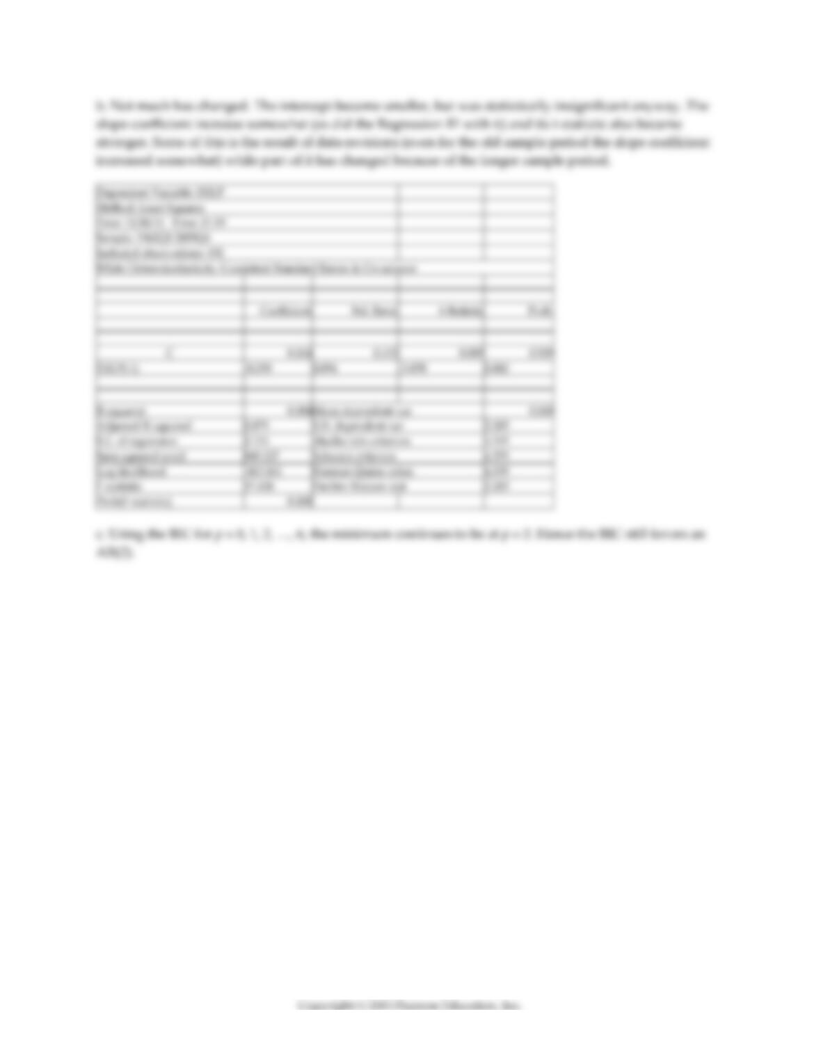
a. Your textbook suggests using two test statistics to test for stationarity: DF and ADF. Test the null
hypothesis that inflation has a stochastic trend against the alternative that it is stationary by performing
the DF and ADF test for a unit autoregressive root. That is, use the equation (14.34) in your textbook with
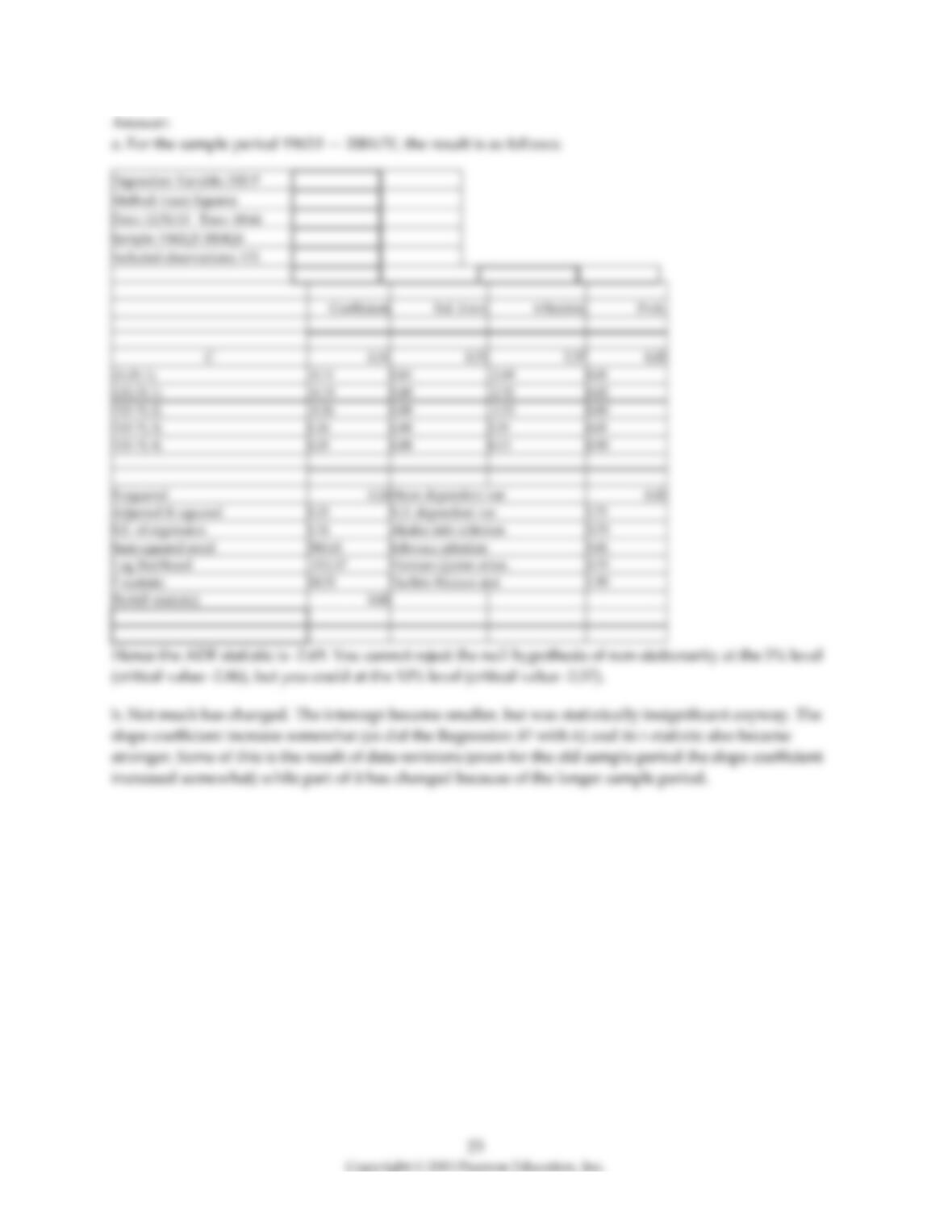
four lags and without a lag of the change in the inflation rate as a regressor for sample period 1962:I —
2004:IV. Go to the Stock and Watson companion website for the textbook and download the data
“Macroeconomic Data Used in Chapters 14 and 16.” Enter the data for consumer price index, calculate the
inflation rate and the acceleration of the inflation rate, and replicate the result on page 526 of your
textbook. Make sure not to use the heteroskedasticity–robust standard error option for the estimation.
b. Next find a website with more recent data, such as the Federal Reserve Economic Data (FRED) site at
the Federal Reserve Bank of St. Louis. Locate the data for the CPI, which will be monthly, and convert the
data in quarterly averages. Then, using a sample from 1962:I — 2009:IV, re–estimate the above
specification and comment on the changes that have occurred.
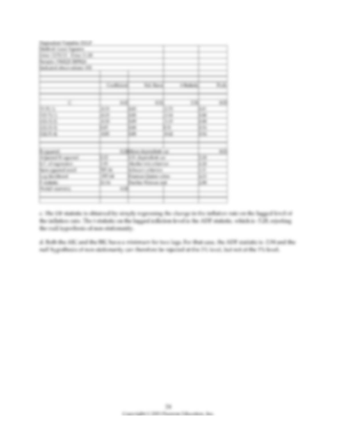
c. For the new sample period, find the DF statistic.
d. Finally, calculate the ADF statistic, allowing for the lag length of the inflation acceleration term to be
determined by either the AIC or the BIC.
14.3 Mathematical and Graphical Problems
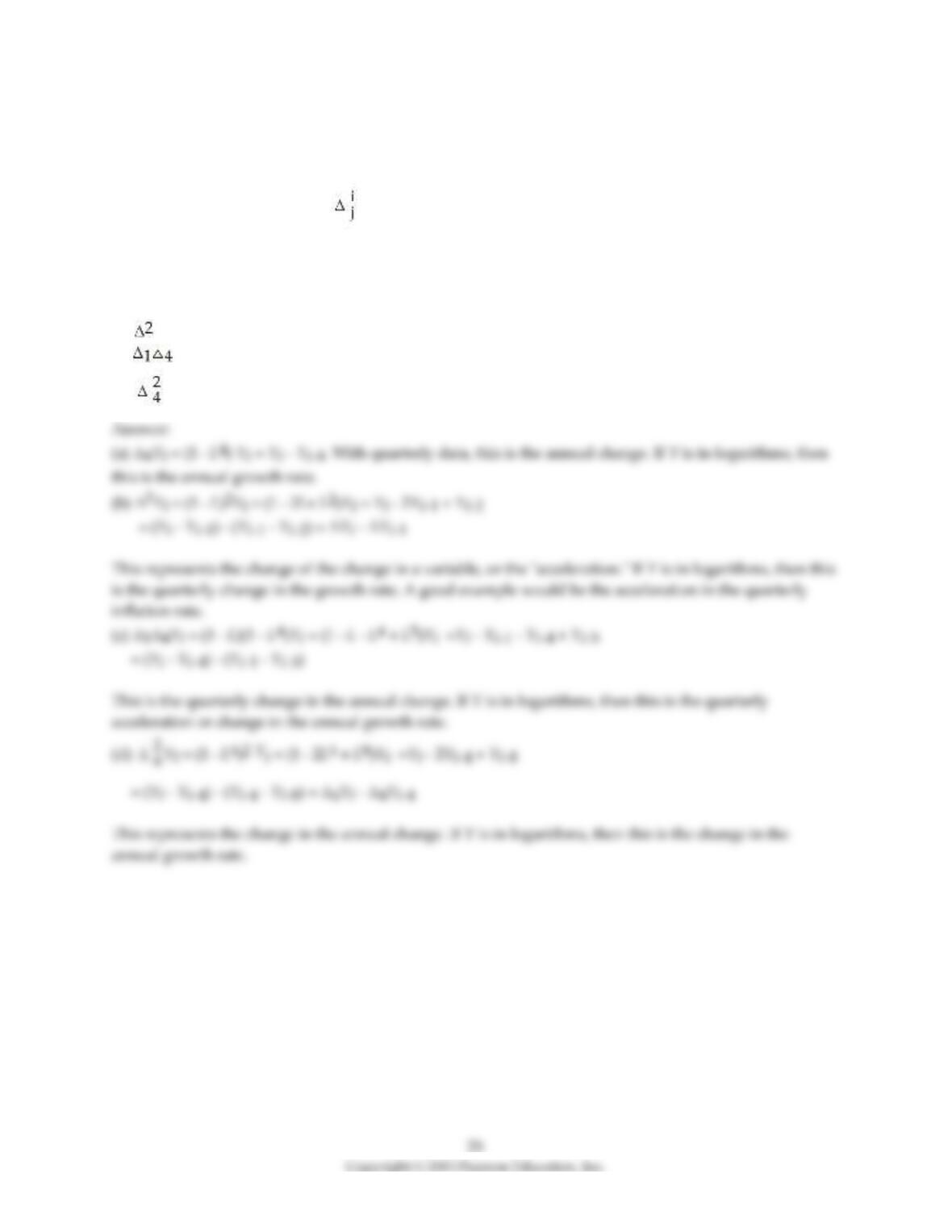
1) (Requires Appendix material) Define the difference operator Δ = (1 – L) where L is the lag operator,
such that LjYt = Yt–j. In general, = (1– Lj)i, where i and j are typically omitted when they take the
value of 1. Show the expressions in Y only when applying the difference operator to the following
expressions, and give the resulting expression an economic interpretation, assuming that you are
working with quarterly data:
(a) Δ4Yt
(b) Yt
(c) Yt
(d) Yt
26
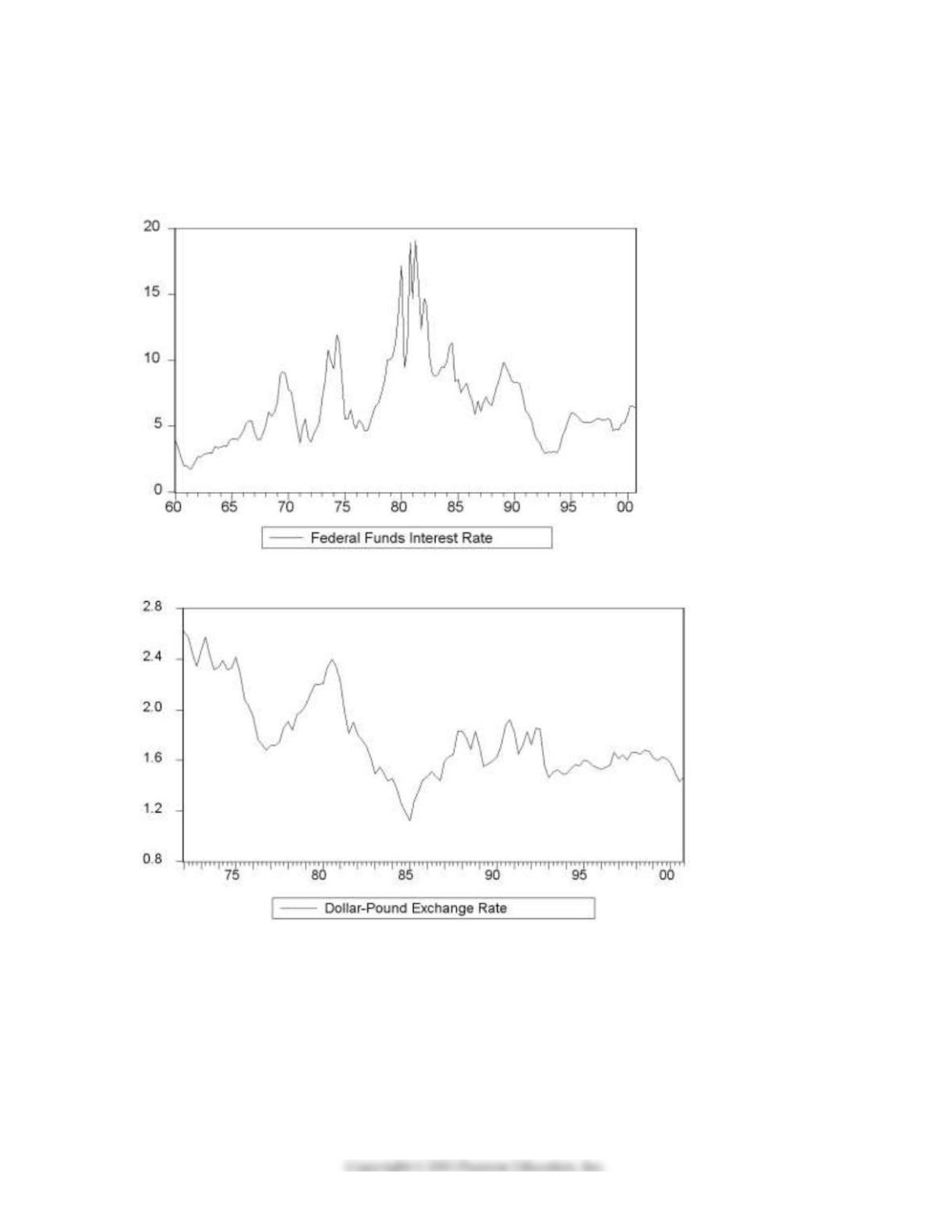
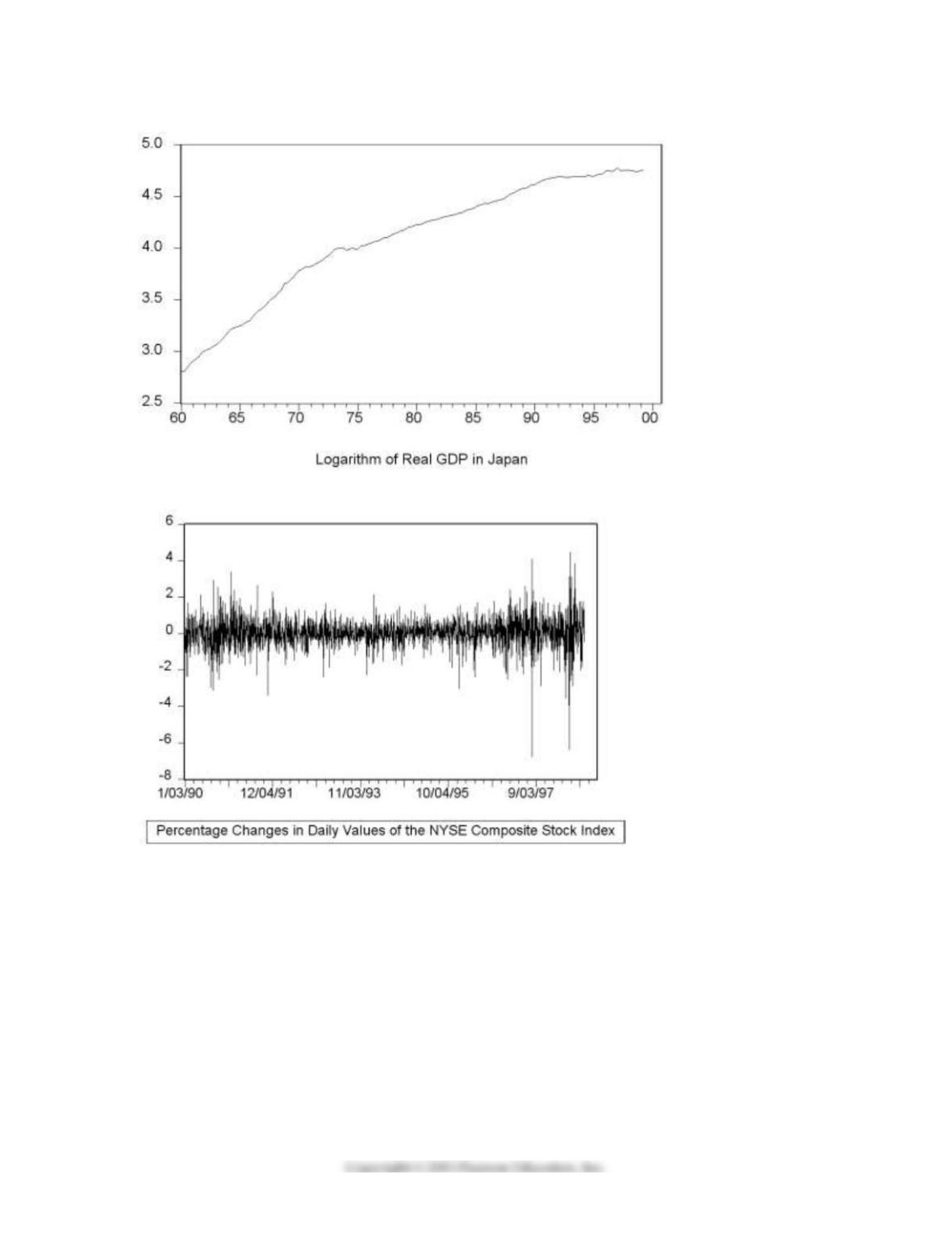
2) The textbook displayed the accompanying four economic time series with “markedly different
patterns.” For each indicate what you think the sample autocorrelations of the level (Y) and change (△Y)
will be and explain your reasoning.
(a)
(b)
27
(c)
(d)


3) You have decided to use the Dickey Fuller (DF) test on the United States aggregate unemployment rate
(sample period 1962:I – 1995:IV). As a result, you estimate the following AR(1) model
t = 0.114 – 0.024 UrateUSt–1, R2 = 0.0118, SER = 0.3417
(0.121) (0.019)
You recall that your textbook mentioned that this form of the AR(1) is convenient because it allows for
you to test for the presence of a unit root by using the t– statistic of the slope. Being adventurous, you
decide to estimate the original form of the AR(1) instead, which results in the following output
t = 0.114 – 0.976 UrateUSt–1, R2 = 0.9510, SER = 0.3417
(0.121) (0.019)
You are surprised to find the constant, the standard errors of the two coefficients, and the SER
unchanged, while the regression R2 increased substantially. Explain this increase in the regression R2.
Why should you have been able to predict the change in the slope coefficient and the constancy of the
standard errors of the two coefficients and the SER?

30
4) Consider the standard AR(1) Yt = β0 + β1Yt–1 + ut, where the usual assumptions hold.
(a) Show that yt = β0Yt–1 + ut, where yt is Yt with the mean removed, i.e., yt = Yt – E(Yt). Show that E(Yt)
= 0.
(b) Show that the r–period ahead forecast E(+r) = . If 0 < β1 < 1, how does the r–period ahead
forecast behave as r becomes large? What is the forecast of for large r?
(c) The median lag is the number of periods it takes a time series with zero mean to halve its current
value (in expectation), i.e., the solution r to E(+r) = 0.5 . Show that in the present case this is given
by r = – .
Answer:
5) Consider the following model
Yt = α0 + α1+ ut
where the superscript “e” indicates expected values. This may represent an example where consumption
depended on expected, or “permanent,” income. Furthermore, let expected income be formed as follows:
= + λ(Xt–1 –); 0 < λ < 1
This particular type of expectation formation is called the “adaptive expectations hypothesis.”
(a) In the above expectation formation hypothesis, expectations are formed at the beginning of the period,
say the 1st of January if you had annual data. Give an intuitive explanation for this process.
(b) Transform the adaptive expectation hypothesis in such a way that the right hand side of the equation
only contains observable variables, i.e., no expectations.
(c) Show that by substituting the resulting equation from the previous question into the original equation,
you get an ADL(0, ∞) type equation. How are the coefficients of the regressors related to each other?
(d) Can you think of a transformation of the ADL(0, ∞) equation into an ADL(1,1) type equation, if you
allowed the error term to be (ut – λut–1)?

32
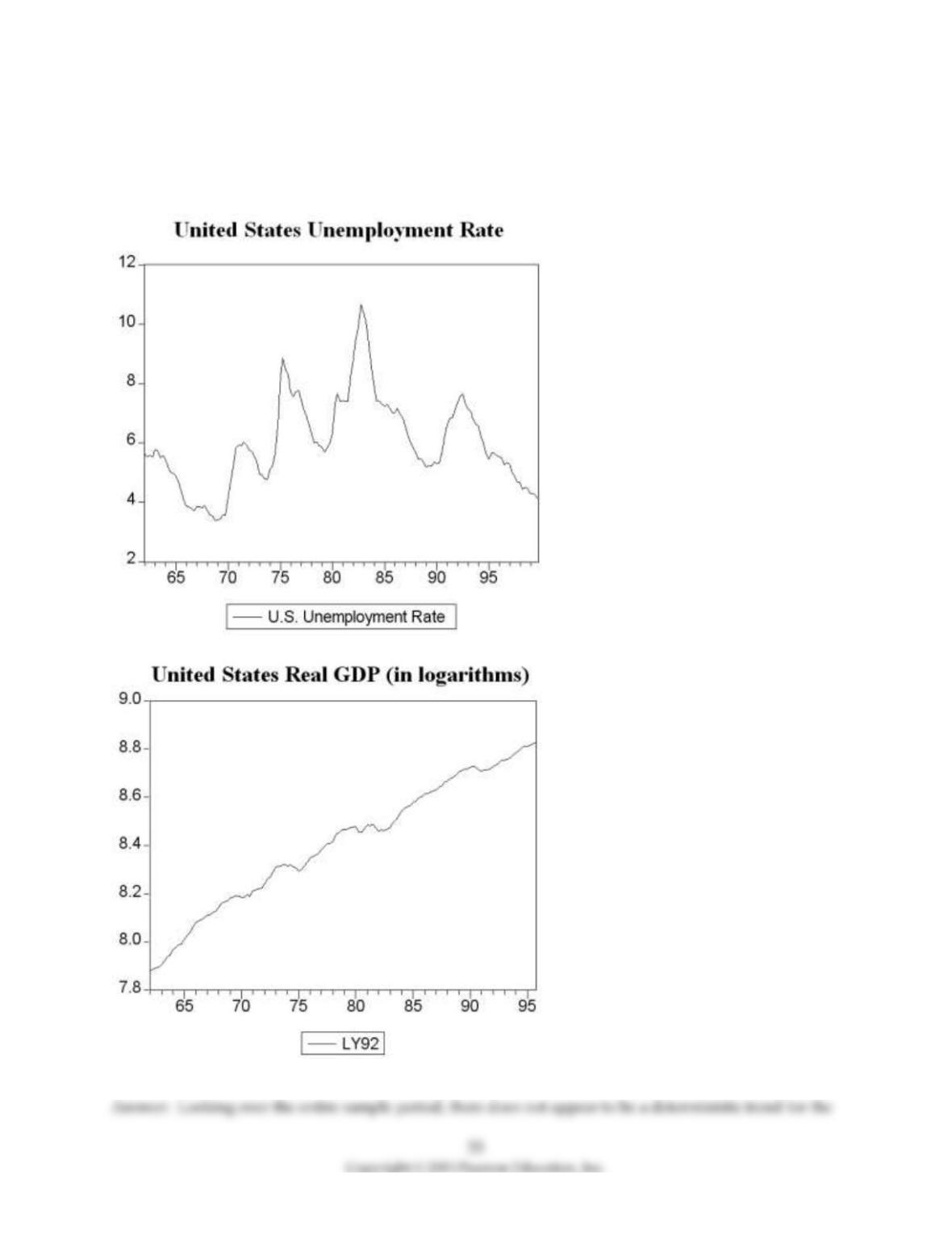
6) The following two graphs give you a plot of the United States aggregate unemployment rate for the
sample period 1962:I to 1999:IV, and the (log) level of real United States GDP for the sample period 1962:I
to 1995:IV. You want test for stationarity in both cases. Indicate whether or not you should include a time
trend in your Augmented Dickey–Fuller test and why.

7) (Requires Appendix material): Show that the AR(1) process Yt = a1Yt–1 + et;< 1, can be converted to
a MA(∞) process.
8) (Requires Appendix material) The long–run, stationary state solution of an AD(p,q) model, which can
be written as A(L)Yt = β0 + c(L)Xt–1 + ut, where = 1, and = –βj, cj = δj, can be found by setting L=1 in
the two lag polynomials. Explain. Derive the long–run solution for the estimated ADL(4,4) of the change
in the inflation rate on unemployment:
t = 1.32 – .36 ΔInft–1 – 0.34vInft–2 + 0.7ΔInft–3 – 0.3ΔInft–4
–2.68Unempt–1 + 3.43Unempt–2 – 1.04Unempt–3 + .07Unempt–4
Assume that the inflation rate is constant in the long–run and calculate the resulting unemployment rate.
What does the solution represent? Is it reasonable to assume that this long–run solution is constant over
the estimation period 1962–1999? If not, how could you detect the instability?
35
9) You want to determine whether or not the unemployment rate for the United States has a stochastic
trend using the Augmented Dickey Fuller Test (ADF). The BIC suggests using 3 lags, while the AIC
suggests 4 lags.
(a) Which of the two will you use for your choice of the optimal lag length?
(b) After estimating the appropriate equation, the t–statistic on the lag level unemployment rate is (–2.186)
(using a constant, but not a trend). What is your decision regarding the stochastic trend of the
unemployment rate series in the United States?
(c) Having worked in the previous exercise with the unemployment rate level, you repeat the exercise
using the difference in United States unemployment rates. Write down the appropriate equation to
conduct the Augmented Dickey–Fuller test here. The t–statistic on relevant coefficient turns out to be (–
4.791). What is your conclusion now?
10) Consider the AR(1) model Yt = β0 + β1Yt–1 + ut, < 1..
(a) Find the mean and variance of Yt.
(b) Find the first two autocovariances of Yt.
(c) Find the first two autocorrelations of Yt.
Answer:
36
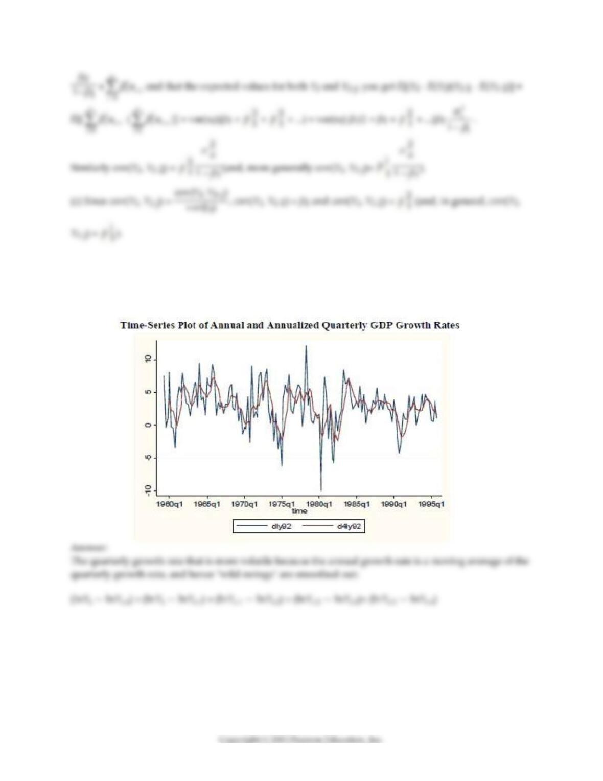
11) Find data for real GDP (Yt) for the United States for the time period 1959:I (first quarter) to 1995:IV.
Next generate two growth rates: The (annualized) quarterly growth rate of real GDP
[(lnYt — lnYt–1) × 400] and the annual growth rate of real GDP [(lnYt — lnYt–4) × 100]. Which is more
volatile? What is the reason for this? Explain.

37
12) You have collected data for real GDP (Y) and have estimated the following function:
ln t = 7.866 + 0.00679×Zeit
(0.007) (0.00008)
t = 1961:I — 2007:IV, R2 = 0.98, SER = 0.036
where Zeit is a deterministic time trend, which takes on the value of 1 during the first quarter of 1961,
and is increased by one for each following quarter.
a. Interpret the slope coefficient. Does it make sense?
b. Interpret the regression R2. Are you impressed by its value?
c. Do you think that given the regression R2, you should use the equation to forecast real GDP beyond
the sample period?