7) Studies of the effect of minimum wages on teenage employment typically regress the teenage
employment to population ratio on the real minimum wage or the minimum wage relative to average
hourly earnings using OLS. Assume that you have a cross section of United States for two years. Do you
think that there are problems with simultaneous equation bias?
13
12.3 Mathematical and Graphical Problems
1) To analyze the year–to–year variation in temperature data for a given city, you regress the daily high
temperature (Temp) for 100 randomly selected days in two consecutive years (1997 and 1998) for Phoenix.
The results are (heteroskedastic–robust standard errors in parenthesis):
= 15.63 + 0.80 × ; R2= 0.65, SER = 9.63
(0.10)
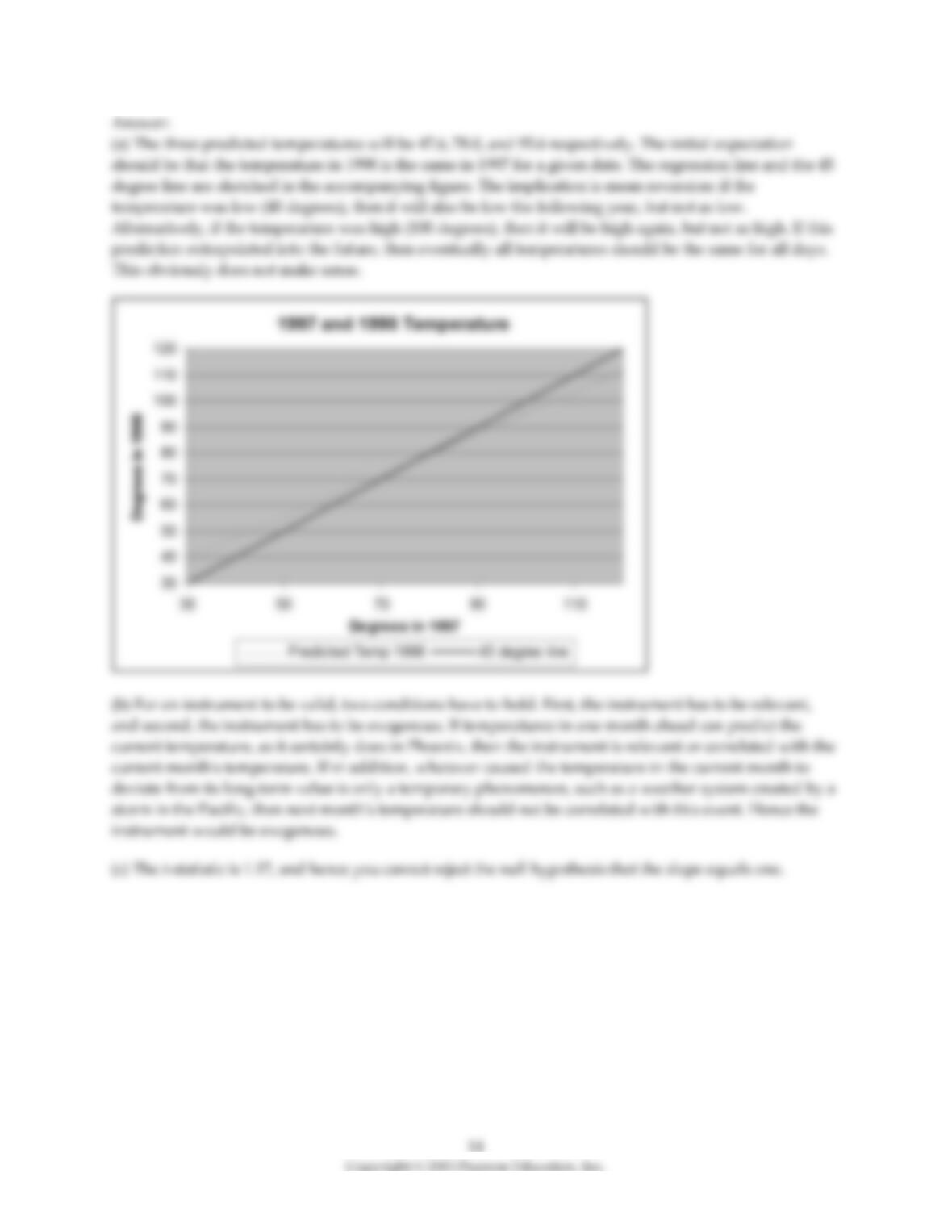
(a) Calculate the predicted temperature for the current year if the temperature in the previous year was
40°F, 78°F, and 100°F. How does this compare with you prior expectation? Sketch the regression line and
compare it to the 45 degree line. What are the implications?
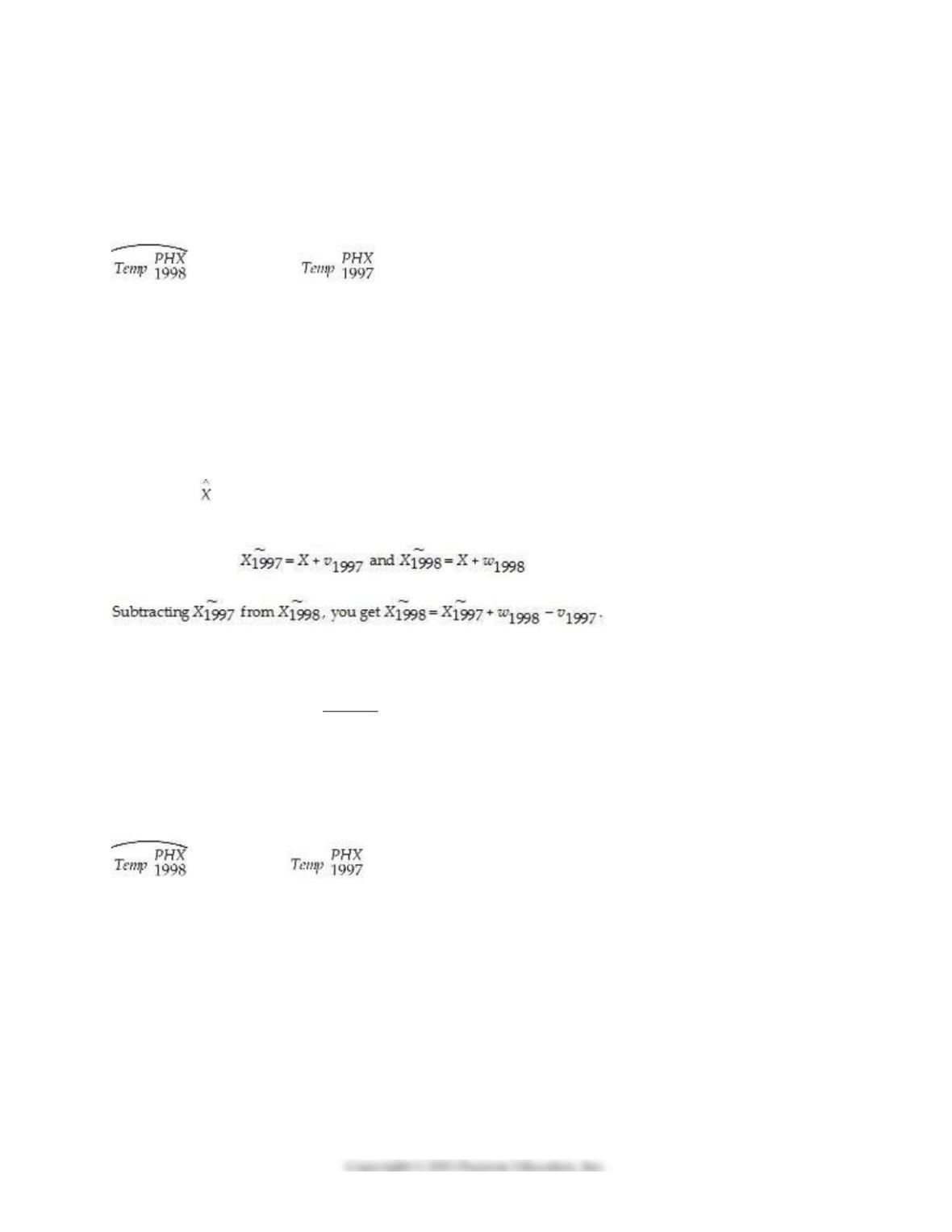
(b) You recall having studied errors–in–variables before. Although the web site you received your data
from seems quite reliable in measuring data accurately, what if the temperature contained measurement
error in the following sense: for any given day, say January 28, there is a true underlying seasonal
temperature (X), but each year there are different temporary weather patterns (v, w) which result in a
temperature different from X. For the two years in your data set, the situation can be described as
follows:
Hence the population parameter
for the intercept and slope are zero and one, as expected. It is not difficult to show that the OLS estimator
for the slope is inconsistent, where
2
122
ˆ1
pv
xv
⎯⎯→ − +
As a result you consider estimating the slope and intercept by TSLS. You think about an instrument and
consider the temperature one month ahead of the observation in the previous year. Discuss instrument
validity for this case.
(c) The TSLS estimation result is as follows:
= –6.24 + 1.07×;
(0.06)
Perform a t–test on whether or not the slope is now significantly different from one.
2) Consider the following population regression model relating the dependent variable Yi and regressor
Xi,
Yi = β0 + β1Xi + ui, i = 1, …, n.
Xi ≡ Yi + Zi
where Z is a valid instrument for X.
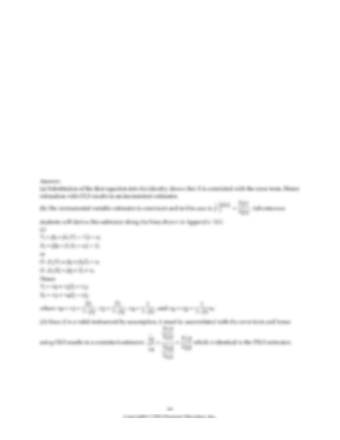
(a) Explain why you should not use OLS to estimate β1.
(b) To generate a consistent estimator for β1, what should you do?
(c) The two equations above make up a system of equations in two unknowns. Specify the two reduced
form equations in terms of the original coefficients. (Hint: substitute the identity into the first equation
and solve for Y. Similarly, substitute Y into the identity and solve for X.)
(d) Do the two reduced form equations satisfy the OLS assumptions? If so, can you find consistent
estimators of the two slopes? What is the ratio of the two estimated slopes? This estimator is called
“Indirect Least Squares.” How does it compare to the TSLS in this example?
3) Here are some examples of the instrumental variables regression model. In each case you are given the
number of instruments and the J–statistic. Find the relevant value from the distribution, using a 1%
and 5% significance level, and make a decision whether or not to reject the null hypothesis.
(a) Yi = β0 + β1X1i + ui, i = 1, …, n; Z1i, Z2i are valid instruments, J = 2.58.
(b) Yi = β0 + β1X1i + β2X2i + β3W1i + ui, i = 1, …, n; Z1i, Z2i, Z3i, Z4i are valid instruments, J = 9.63.
(c) Yi = β0 + β1X1i + β2W1i + β3W2i + β4W3i + ui, i = 1, …, n; Z1i, Z2i, Z3i, Z4i are valid instruments, J =
11.86.
4) To study the determinants of growth between the countries of the world, researchers have used panels
of countries and observations spanning over long periods of time (e.g. 1965–1975, 1975–1985, 1985–1990).
Some of these studies have focused on the effect that inflation has on growth and found that although the
effect is small for a given time period, it accumulates over time and therefore has an important negative
effect.
(a) Explain why the OLS estimator may be biased in this case.
(b) Explain how methods using panel data could potentially alleviate the problem.
(c) Some authors have suggested using an index of central bank independence as an instrumental.
Discuss whether or not such an index would be a valid instrument.
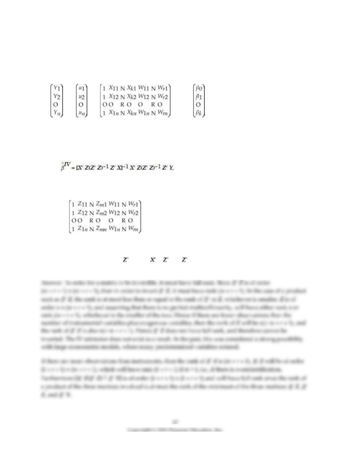
5) (Requires Matrix Algebra) The population multiple regression model can be written in matrix form as
Y = Xβ + U
where
Y = , U = , X = , and β =
Note that the X matrix contains both k endogenous regressors and (r +1) included exogenous regressors
(the constant is obviously exogenous).
The instrumental variable estimator for the overidentified case is
where Z is a matrix, which contains two types of variables: first the r included exogenous regressors plus
the constant, and second, m instrumental variables.
Z =
It is of order n × (m+r+1).
For this estimator to exist, both ( Z) and [ Z( Z)–1 X] must be invertible. State the conditions
under which this will be the case and relate them to the degree of overidentification.
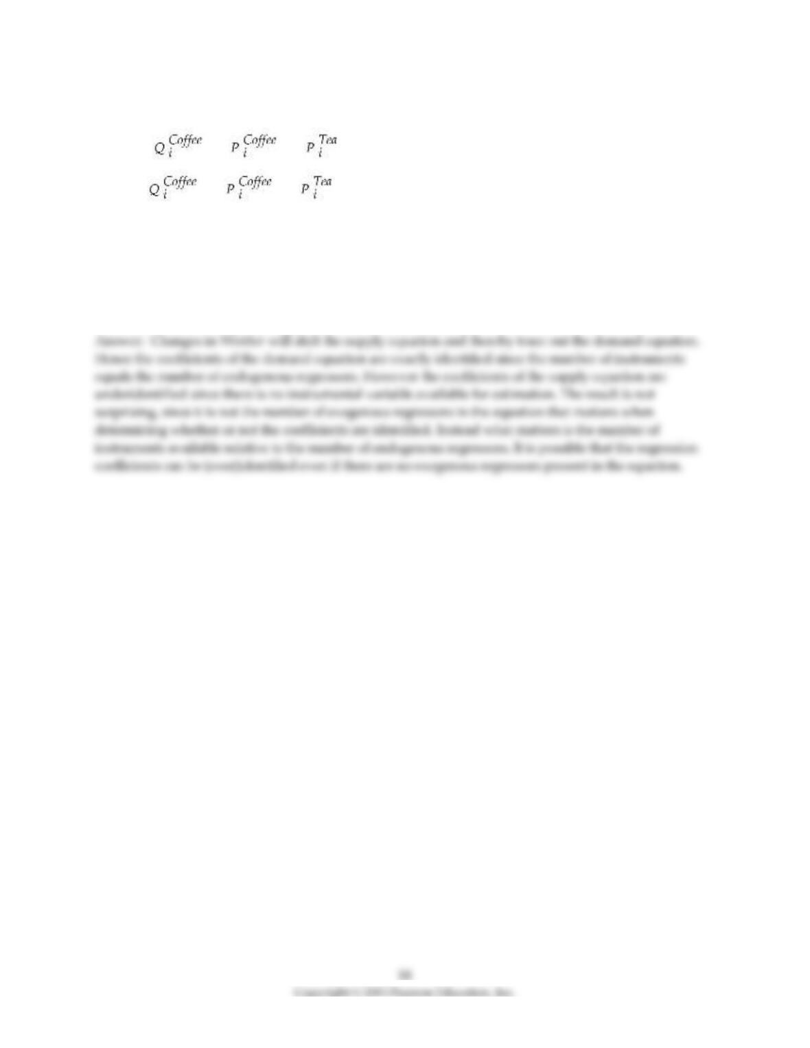
6) Consider the following model of demand and supply of coffee:
Demand: = β1 + β2 + ui
Supply: = β3 + β4 + β5Weather + vi
(variables are measure in deviations from means, so that the constant is omitted).
What are the expected signs of the various coefficients this model? Assume that the price of tea and
Weather are exogenous variables. Are the coefficients in the supply equation identified? Are the
coefficients in the demand equation identified? Are they overidentified? Is this result surprising given
that there are more exogenous regressors in the second equation?
7) You started your econometrics course by studying the OLS estimator extensively, first for the simple
regression case and then for extensions of it. You have now learned about the instrumental variable
estimator. Under what situation would you prefer one to the other? Be specific in explaining under which
situations one estimation method generates superior results.
8) Your textbook gave an example of attempting to estimate the demand for a good in a market, but being
unable to do so because the demand function was not identified. Is this the case for every market?
Consider, for example, the demand for sports events. One of your peers estimated the following demand
function after collecting data over two years for every one of the 162 home games of the 2000 and 2001
season for the Los Angeles Dodgers.
= 15,005 + 201 × Temperat + 465 × DodgNetWin + 82 × OppNetWin
(8,770) (121) (169) (26)
+ 9647 × DFSaSu + 1328 × Drain + 1609 × D150m + 271 × DDiv – 978 × D2001;
(1505) (3355) (1819) (1,184) (1,143)
R2 = 0.416, SER = 6983
Where Attend is announced stadium attendance, Temperat it the average temperature on game day,
DodgNetWin are the net wins of the Dodgers before the game (wins–losses), OppNetWin is the opposing
team’s net wins at the end of the previous season, and DFSaSu, Drain, D150m, Ddiv, and D2001 are binary
variables, taking a value of 1 if the game was played on a weekend, it rained during that day, the
opposing team was within a 150 mile radius, plays in the same division as the Dodgers, and during 2001,
respectively. Numbers in parenthesis are heteroskedasticity– robust standard errors.
Even if there is no identification problem, is it likely that all regressors are uncorrelated with the error
term? If not, what are the consequences?
9) Earnings functions, whereby the log of earnings is regressed on years of education, years of on the job
training, and individual characteristics, have been studied for a variety of reasons. Some studies have
focused on the returns to education, others on discrimination, union non–union differentials, etc. For all
these studies, a major concern has been the fact that ability should enter as a determinant of earnings, but
that it is close to impossible to measure and therefore represents an omitted variable.
Assume that the coefficient on years of education is the parameter of interest. Given that education is
positively correlated to ability, since, for example, more able students attract scholarships and hence
receive more years of education, the OLS estimator for the returns to education could be upward biased.
To overcome this problem, various authors have used instrumental variable estimation techniques. For
each of the instruments potential instruments listed below briefly discuss instrument validity.
(a) The individual’s postal zip code.
(b) The individual’s IQ or testscore on a work related exam.
(c) Years of education for the individual’s mother or father.
(d) Number of siblings the individual has.
10) The two conditions for instrument validity are corr(Zi, Xi) ≠ 0 and corr(Zi, ui) = 0. The reason for the
inconsistency of OLS is that corr(Xi, ui) ≠ 0. But if X and Z are correlated, and X and u are also correlated,
then how can Z and u not be correlated? Explain.
11) Consider the a model of the U.S. labor market where the demand for labor depends on the real wage,
while the supply of labor is vertical and does not depend on the real wage. You could argue that the
supply of labor by households (think of hours supplied by two adults and two children) has not changed
much over the last 60 years or so in the U.S. while real wages more than doubled over the same time
span. At first that seems strange given the higher participation rate of females over that period, but that
increase has been countered by a lower male participation rate (resulting from earlier retirement), an
increase in legal holidays, and an increase in vacation days.
a. Write down two equations representing the labor supply and labor demand function, allowing for an
error term in each of the demand and supply equation. In addition, assume that the labor market clears.
b. How would you estimate the labor supply equation?
c. Assuming that the error terms are mutually independent i.i.d. random variables, both with mean
zero, show that the real wage and the error term of the labor demand equation are correlated.
d. If you find a non–zero correlation, should you estimate the labor demand equation using OLS? If so,
what are the consequences?
e. Estimating the labor demand equation by IV estimation, which instrument suggests itself
immediately?