
Introduction to Econometrics, 3e (Stock)
Chapter 11 Regression with a Binary Dependent Variable
11.1 Multiple Choice
1) The binary dependent variable model is an example of a
A) regression model, which has as a regressor, among others, a binary variable.
B) model that cannot be estimated by OLS.
C) limited dependent variable model.
D) model where the left–hand variable is measured in base 2.
2) (Requires Appendix material) The following are examples of limited dependent variables, with the
exception of
A) binary dependent variable.
B) log–log specification.
C) truncated regression model.
D) discrete choice model.
3) In the binary dependent variable model, a predicted value of 0.6 means that
A) the most likely value the dependent variable will take on is 60 percent.
B) given the values for the explanatory variables, there is a 60 percent probability that the dependent
variable will equal one.
C) the model makes little sense, since the dependent variable can only be 0 or 1.
D) given the values for the explanatory variables, there is a 40 percent probability that the dependent
variable will equal one.
4) E(Y X1, …, Xk) = Pr(Y = 1 X1,…, Xk) means that
A) for a binary variable model, the predicted value from the population regression is the probability that
Y=1, given X.
B) dividing Y by the X‘s is the same as the probability of Y being the inverse of the sum of the X‘s.
C) the exponential of Y is the same as the probability of Y happening.
D) you are pretty certain that Y takes on a value of 1 given the X‘s.
5) The linear probability model is
A) the application of the multiple regression model with a continuous left–hand side variable and a
binary variable as at least one of the regressors.
B) an example of probit estimation.
C) another word for logit estimation.
D) the application of the linear multiple regression model to a binary dependent variable.

6) In the linear probability model, the interpretation of the slope coefficient is
A) the change in odds associated with a unit change in X, holding other regressors constant.
B) not all that meaningful since the dependent variable is either 0 or 1.
C) the change in probability that Y=1 associated with a unit change in X, holding others regressors
constant.
D) the response in the dependent variable to a percentage change in the regressor.
7) The following tools from multiple regression analysis carry over in a meaningful manner to the linear
probability model, with the exception of the
A) F–statistic.
B) significance test using the t–statistic.
C) 95% confidence interval using ± 1.96 times the standard error.
D) regression R2.
8) (Requires material from Section 11.3 – possibly skipped) For the measure of fit in your regression
model with a binary dependent variable, you can meaningfully use the
A) regression R2.
B) size of the regression coefficients.
C) pseudo R2.
D) standard error of the regression.
9) The major flaw of the linear probability model is that
A) the actuals can only be 0 and 1, but the predicted are almost always different from that.
B) the regression R2 cannot be used as a measure of fit.
C) people do not always make clear–cut decisions.
D) the predicted values can lie above 1 and below 0.
10) The probit model
A) is the same as the logit model.
B) always gives the same fit for the predicted values as the linear probability model for values between
0.1 and 0.9.
C) forces the predicted values to lie between 0 and 1.
D) should not be used since it is too complicated.
11) The logit model derives its name from
A) the logarithmic model.
B) the probit model.
C) the logistic function.
D) the tobit model.

12) In the probit model Pr(Y = 1 = Φ(β0 + β1X), Φ
A) is not defined for Φ(0).
B) is the standard normal cumulative distribution function.
C) is set to 1.96.
D) can be computed from the standard normal density function.
13) In the expression Pr(Y = 1 = Φ(β0 + β1X),
A) (β0 + β1X) plays the role of z in the cumulative standard normal distribution function.
B) β1 cannot be negative since probabilities have to lie between 0 and 1.
C) β0 cannot be negative since probabilities have to lie between 0 and 1.
D) min (β0 + β1X) > 0 since probabilities have to lie between 0 and 1.
14) In the probit model Pr(Y = 1 X1, X2,…, Xk) = Φ(β0 + β1X1 + βxX2 + … + βkXk),
A) the β‘s do not have a simple interpretation.
B) the slopes tell you the effect of a unit increase in X on the probability of Y.
C) β0 cannot be negative since probabilities have to lie between 0 and 1.
D) β0 is the probability of observing Y when all X‘s are 0
15) In the expression Pr(deny = 1 P/I Ratio, black) = Φ(–2.26 + 2.74P/I ratio + 0.71black), the effect of
increasing the P/I ratio from 0.3 to 0.4 for a white person
A) is 0.274 percentage points.
B) is 6.1 percentage points.
C) should not be interpreted without knowledge of the regression R2.
D) is 2.74 percentage points.
16) The maximum likelihood estimation method produces, in general, all of the following desirable
properties with the exception of
A) efficiency.
B) consistency.
C) normally distributed estimators in large samples.
D) unbiasedness in small samples.
17) The logit model can be estimated and yields consistent estimates if you are using
A) OLS estimation.
B) maximum likelihood estimation.
C) differences in means between those individuals with a dependent variable equal to one and those with
a dependent variable equal to zero.
D) the linear probability model.

18) When having a choice of which estimator to use with a binary dependent variable, use
A) probit or logit depending on which method is easiest to use in the software package at hand.
B) probit for extreme values of X and the linear probability model for values in between.
C) OLS (linear probability model) since it is easier to interpret.
D) the estimation method which results in estimates closest to your prior expectations.
19) Nonlinear least squares
A) solves the minimization of the sum of squared predictive mistakes through sophisticated
mathematical routines, essentially by trial and error methods.
B) should always be used when you have nonlinear equations.
C) gives you the same results as maximum likelihood estimation.
D) is another name for sophisticated least squares.
20) (Requires Advanced material) Only one of the following models can be estimated by OLS:
A) Y = AKαLβ + u.
B) Pr(Y = 1 X) = Φ(β0 + β1X)
C) Pr(Y = 1 X) = F(β0 + β1X) = .
D) Y = AKα Lβu.
21) (Requires Advanced material) Nonlinear least squares estimators in general are not
A) consistent.
B) normally distributed in large samples.
C) efficient.
D) used in econometrics.
22) (Requires Advanced material) Maximum likelihood estimation yields the values of the coefficients
that
A) minimize the sum of squared prediction errors.
B) maximize the likelihood function.
C) come from a probability distribution and hence have to be positive.
D) are typically larger than those from OLS estimation.
23) To measure the fit of the probit model, you should:
A) use the regression R2.
B) plot the predicted values and see how closely they match the actuals.
C) use the log of the likelihood function and compare it to the value of the likelihood function.
D) use the fraction correctly predicted or the pseudo R2.

24) When estimating probit and logit models,
A) the t–statistic should still be used for testing a single restriction.
B) you cannot have binary variables as explanatory variables as well.
C) F–statistics should not be used, since the models are nonlinear.
D) it is no longer true that the 2 < R2.
25) The following problems could be analyzed using probit and logit estimation with the exception of
whether or not
A) a college student decides to study abroad for one semester.
B) being a female has an effect on earnings.
C) a college student will attend a certain college after being accepted.
D) applicants will default on a loan.
26) In the probit regression, the coefficient β1 indicates
A) the change in the probability of Y = 1 given a unit change in X
B) the change in the probability of Y = 1 given a percent change in X
C) the change in the z– value associated with a unit change in X
D) none of the above
27) Your textbook plots the estimated regression function produced by the probit regression of deny on
P/I ratio. The estimated probit regression function has a stretched “S” shape given that the coefficient on
the P/I ratio is positive. Consider a probit regression function with a negative coefficient. The shape would
A) resemble an inverted “S” shape (for low values of X, the predicted probability of Y would approach 1)
B) not exist since probabilities cannot be negative
C) remain the “S” shape as with a positive slope coefficient
D) would have to be estimated with a logit function
28) Probit coefficients are typically estimated using
A) the OLS method
B) the method of maximum likelihood
C) non–linear least squares (NLLS)
D) by transforming the estimates from the linear probability model
29) F–statistics computed using maximum likelihood estimators
A) cannot be used to test joint hypothesis
B) are not meaningful since the entire regression R2 concept is hard to apply in this situation
C) do not follow the standard F distribution
D) can be used to test joint hypothesis

30) When testing joint hypothesis, you can use
A) the F– statistic
B) the chi–squared statistic
C) either the F–statistic or the chi–square statistic
D) none of the above
11.2 Essays and Longer Questions
1) Your task is to model students’ choice for taking an additional economics course after the first
principles course. Describe how to formulate a model based on data for a large sample of students.
Outline several estimation methods and their relative advantage over other methods in tackling this
problem. How would you go about interpreting the resulting output? What summary statistics should be
included?
7
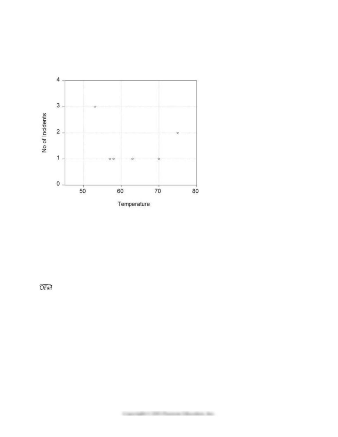
2) The Report of the Presidential Commission on the Space Shuttle Challenger Accident in 1986 shows a plot of
the calculated joint temperature in Fahrenheit and the number of O–rings that had some thermal distress.
You collect the data for the seven flights for which thermal distress was identified before the fatal flight
and produce the accompanying plot.
(a) Do you see any relationship between the temperature and the number of O–ring failures? If you fitted
a linear regression line through these seven observations, do you think the slope would be positive or
negative? Significantly different from zero? Do you see any problems other than the sample size in your
procedure?
(b) You decide to look at all successful launches before Challenger, even those for which there were no
incidents. Furthermore you simplify the problem by specifying a binary variable, which takes on the
value one if there was some O–ring failure and is zero otherwise. You then fit a linear probability model
with the following result,
= 2.858 – 0.037 × Temperature; R2 = 0.325, SER = 0.390,
(0.496) (0.007)
where Ofail is the binary variable which is one for launches where O–rings showed some thermal distress,
and Temperature is measured in degrees of Fahrenheit. The numbers in parentheses are
heteroskedasticity–robust standard errors.
Interpret the equation. Why do you think that heteroskedasticity–robust standard errors were used? What
is your prediction for some O–ring thermal distress when the temperature is 31°, the temperature on
January 28, 1986? Above which temperature do you predict values of less than zero? Below which
temperature do you predict values of greater than one?
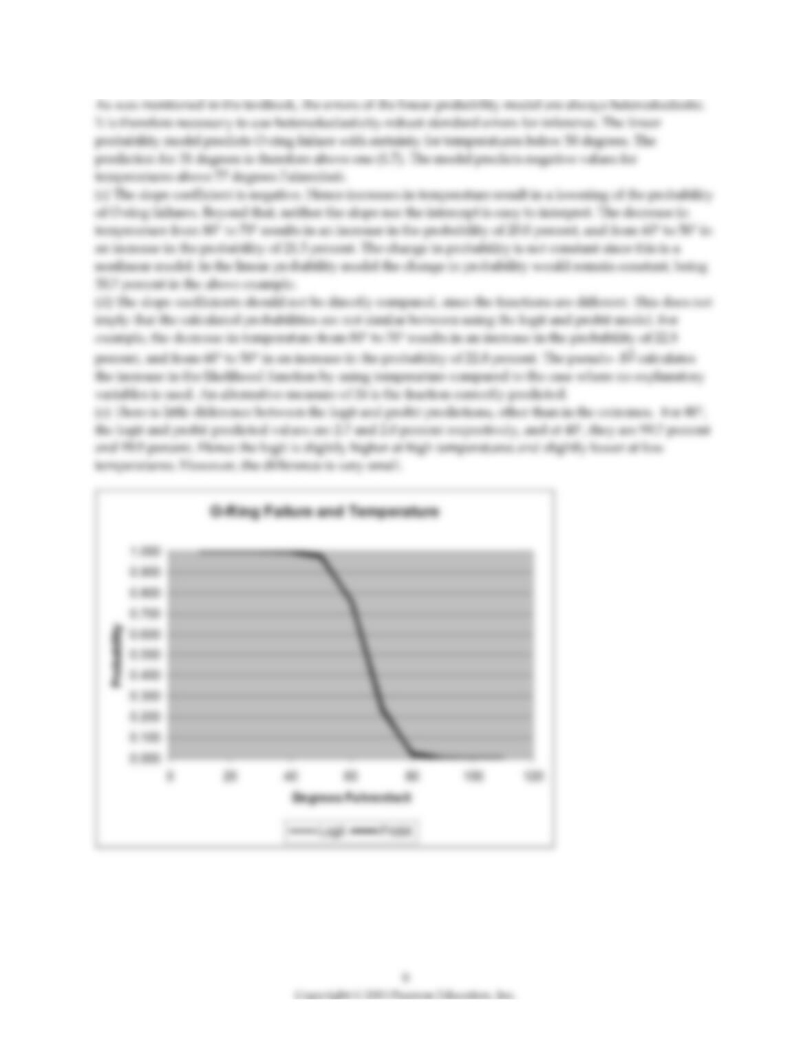
(c) To fix the problem encountered in (b), you re–estimate the relationship using a logit regression:

Pr(OFail = 1 Temperature) = F (15.297 – 0.236 × Temperature); pseudo– R2=0.297
(7.329) (0.107)
What is the meaning of the slope coefficient? Calculate the effect of a decrease in temperature from 80° to
70°, and from 60° to 50°. Why is the change in probability not constant? How does this compare to the
linear probability model?
(d) You want to see how sensitive the results are to using the logit, rather than the probit estimation
method. The probit regression is as follows:
Pr(OFail = 1 Temperature) = Φ(8.900 – 0.137 × Temperature); pseudo– R2=0.296
(3.983) (0.058)
Why is the slope coefficient in the probit so different from the logit coefficient? Calculate the effect of a
decrease in temperature from 80° to 70°, and from 60° to 50° and compare the resulting changes in
probability to your results in (c). What is the meaning of the pseudo– R2? What other measures of fit
might you want to consider?
(e) Calculate the predicted probability for 80° and 40°, using your probit and logit estimates. Based on the
relationship between the probabilities, sketch what the general relationship between the logit and probit
regressions is. Does there seem to be much of a difference for values other than these extreme values?
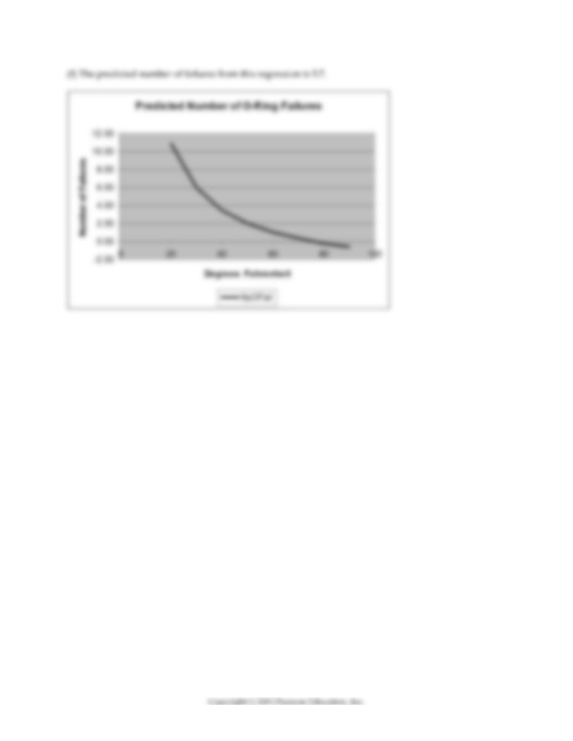
(f) You decide to run one more regression, where the dependent variable is the actual number of
incidences (NoOFail). You allow for a different functional form by choosing the inverse of the
temperature, and estimate the regression by OLS.
= –3.8853 + 295.545 × (1/Temperature); R2 = 0.386, SER = 0.622
(1.516) (106.541)
What is your prediction for O–ring failures for the 31° temperature which was forecasted for the launch
on January 28, 1986? Sketch the fitted line of the regression above.
10

11
3) A study tried to find the determinants of the increase in the number of households headed by a female.
Using 1940 and 1960 historical census data, a logit model was estimated to predict whether a woman is
the head of a household (living on her own) or whether she is living within another’s household. The
limited dependent variable takes on a value of one if the female lives on her own and is zero if she shares
housing. The results for 1960 using 6,051 observations on prime–age whites and 1,294 on nonwhites were
as shown in the table:
Regression
(1) White
(2) Nonwhite
Regression model
Logit
Logit
Constant
1.459
(0.685)
–2.874
(1.423)
Age
–0.275
(0.037)
0.084
(0.068)
age squared
0.00463
(0.00044)
0.00021
(0.00081)
education
–0.171
(0.026)
–0.127
(0.038)
farm status
–0.687
(0.173)
–0.498
(0.346)
South
0.376
(0.098)
–0.520
(0.180)
expected family
earnings
0.0018
(0.00019)
0.0011
(0.00024)
family composition
4.123
(0.294)
2.751
(0.345)
Pseudo–R2
0.266
0.189
Percent Correctly
Predicted
82.0
83.4
where age is measured in years, education is years of schooling of the family head, farm status is a binary
variable taking the value of one if the family head lived on a farm, south is a binary variable for living in a
certain region of the country, expected family earnings was generated from a separate OLS regression to
predict earnings from a set of regressors, and family composition refers to the number of family members
under the age of 18 divided by the total number in the family.

The mean values for the variables were as shown in the table.
Variable
(1) White mean
(2) Nonwhite mean
age
46.1
42.9
age squared
2,263.5
1,965.6
education
12.6
10.4
farm status
0.03
0.02
south
0.3
0.5
expected family earnings
2,336.4
1,507.3
family composition
0.2
0.3
(a) Interpret the results. Do the coefficients have the expected signs? Why do you think age was entered
both in levels and in squares?
(b) Calculate the difference in the predicted probability between whites and nonwhites at the sample
mean values of the explanatory variables. Why do you think the study did not combine the observations
and allowed for a nonwhite binary variable to enter?
(c) What would be the effect on the probability of a nonwhite woman living on her own, if education and
family composition were changed from their current mean to the mean of whites, while all other variables
were left unchanged at the nonwhite mean values?

13
4) A study investigated the impact of house price appreciation on household mobility. The underlying
idea was that if a house were viewed as one part of the household’s portfolio, then changes in the value of
the house, relative to other portfolio items, should result in investment decisions altering the current
portfolio. Using 5,162 observations, the logit equation was estimated as shown in the table, where the
limited dependent variable is one if the household moved in 1978 and is zero if the household did not
move:
Regression
model
Logit
constant
–3.323
(0.180)
Male
–0.567
(0.421)
Black
–0.954
(0.515)
Married78
0.054
(0.412)
marriage
change
0.764
(0.416)
A7983
–0257
(0.921)
PURN
–4.545
(3.354)
Pseudo–R2
0.016
where male, black, married78, and marriage change are binary variables. They indicate, respectively, if the
entity was a male–headed household, a black household, was married, and whether a change in marital
status occurred between 1977 and 1978. A7983 is the appreciation rate for each house from 1979 to 1983
minus the SMSA–wide rate of appreciation for the same time period, and PNRN is a predicted
appreciation rate for the unit minus the national average rate.
(a) Interpret the results. Comment on the statistical significance of the coefficients. Do the slope
coefficients lend themselves to easy interpretation?
(b) The mean values for the regressors are as shown in the accompanying table.
Variable
Mean
male
0.82
black
0.09
married78
0.78
marriage change
0.03
A7983
0.003
PNRN
0.007

Taking the coefficients at face value and using the sample means, calculate the probability of a household
moving.
(c) Given this probability, what would be the effect of a decrease in the predicted appreciation rate
of 20 percent, that is A7983 = –0.20?

5) A study analyzed the probability of Major League Baseball (MLB) players to “survive” for another
season, or, in other words, to play one more season. The researchers had a sample of 4,728 hitters and
3,803 pitchers for the years 1901–1999. All explanatory variables are standardized. The probit estimation
yielded the results as shown in the table:
Regression
(1) Hitters
(2) Pitchers
Regression model
probit
probit
constant
2.010
(0.030)
1.625
(0.031)
number of seasons
played
–0.058
(0.004)
–0.031
(0.005)
performance
0.794
(0.025)
0.677
(0.026)
average performance
0.022
(0.033)
0.100
(0.036)
where the limited dependent variable takes on a value of one if the player had one more season (a
minimum of 50 at bats or 25 innings pitched), number of seasons played is measured in years, performance is
the batting average for hitters and the earned run average for pitchers, and average performance refers to
performance over the career.
(a) Interpret the two probit equations and calculate survival probabilities for hitters and pitchers at the
sample mean. Why are these so high?
(b) Calculate the change in the survival probability for a player who has a very bad year by performing
two standard deviations below the average (assume also that this player has been in the majors for many
years so that his average performance is hardly affected). How does this change the survival probability
when compared to the answer in (a)?
(c) Since the results seem similar, the researcher could consider combining the two samples. Explain in
some detail how this could be done and how you could test the hypothesis that the coefficients are the
same.