CHAPTER 11—PERFORMANCE AND STRATEGY IN
COMPETITIVE MARKETS Key
1. In competitive market equilibrium, social welfare is measured by the:
2. No externalities exist when:
3. A government policy that addresses market failures caused by positive externalities is:
4. The burden of a per unit tax on a product will fall primarily on producers when:
5. A per unit tax will cause output prices to increase least when:
6. Failure by market structure can occur when:
7. In competitive markets:
8. Consumer sovereignty reflects:
9. Competition in the cable television service industry is furnished by:
10. Producer surplus is the:
11. The welfare loss triangle depicts:
12. Profits stemming from market power reflect:
13. Failure by market structure is caused by:
14. Externalities are:
15. Undue market power is indicated when buyer influence results in:
16. Utility price and profit regulation is designed to address:
17. A per unit tax on pollution:
18. From an economic perspective, imposition of a per unit tax is only advantageous if:
19. Society’s right to a clean environment is asserted through:
20. Who pays the economic cost of a tax is answered at the point of tax:
21. The costs of pollution taxes are shared by consumers and producers when:
22. A price ceiling is a costly and seldom used mechanism for:
23. A price floor is a costly and commonly used mechanism for:
24. Economic rents are profits due to:
25. Above-normal returns earned in the time interval that exists between when a favorable influence on industry
demand or cost conditions first transpires and the time when competitor entry or growth finally develops are
called:
26. Social Welfare Concepts. Indicate whether each of the following statements is true or false, and explain
why.
A.
Producer surplus tends to fall as the supply curve becomes more elastic.
B.
Consumer surplus tends to rise as demand becomes more elastic.
C.
The market demand curve indicates the minimum price buyers are willing to pay at each level of production.
D.
The market supply curve indicates the minimum price required by sellers as a group to bring forth production.
E.
Consumer surplus is the amount that consumers are willing to pay for a given good or service above and beyond the amount actually
paid.
becomes more elastic, the amount of producer surplus can be expected to fall.
elastic, the difference between perceived value and market prices tends to diminish, and consumer surplus falls.
False. The market supply demand curve indicates the maximum price buyers are willing to pay to bring forth each level of production.
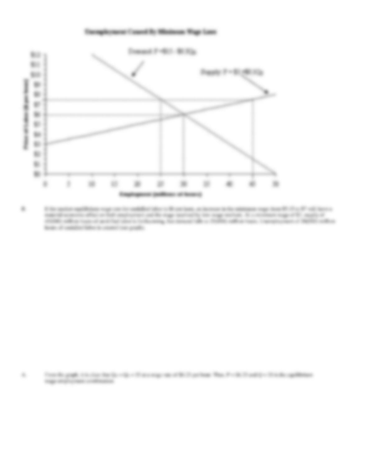
27. Competitive Market Equilibrium. Suppose demand and supply conditions in the competitive market for
unskilled labor are as follows:
QD
= 66.25 – 5P
(Demand)
QS
= -27.5 + 10P
(Supply)
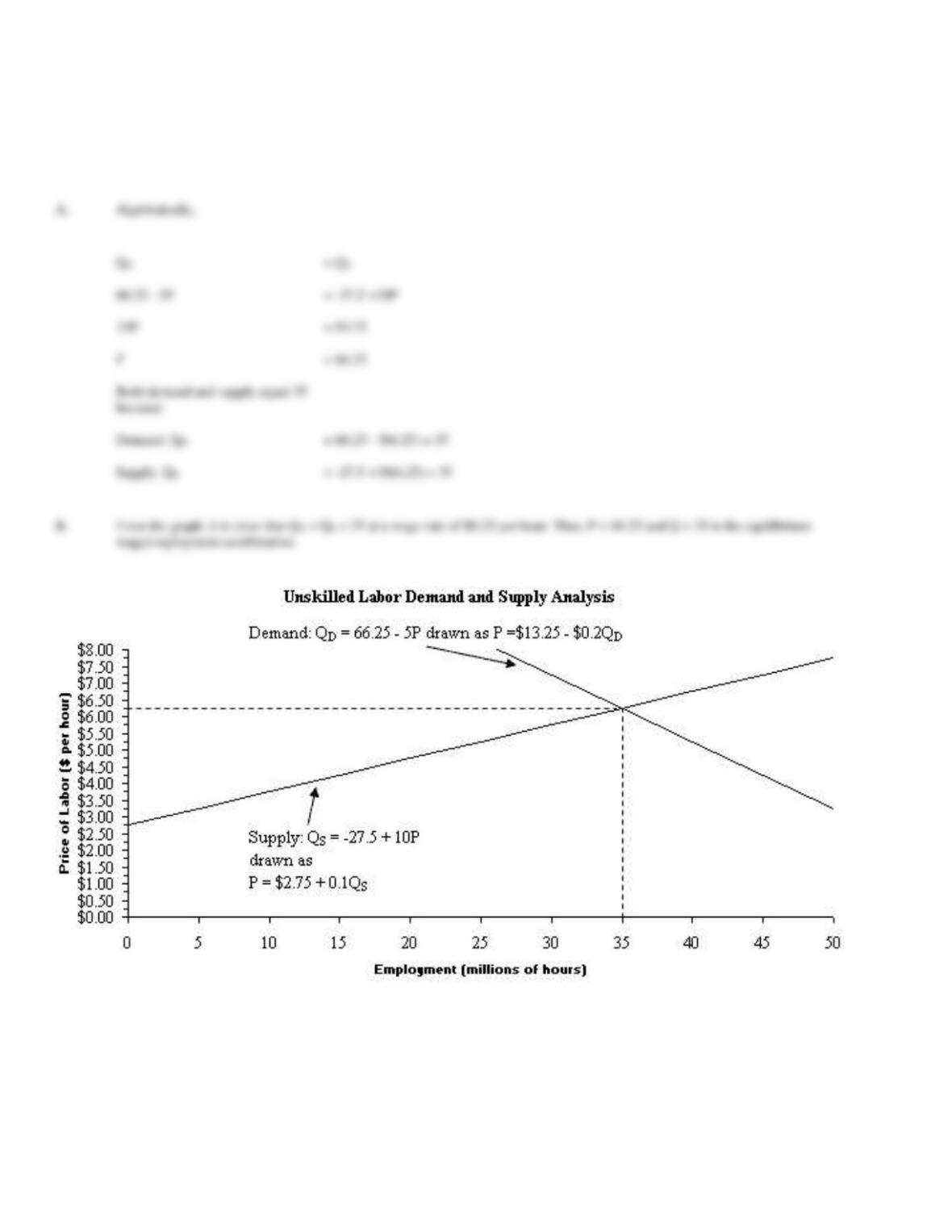
where Q is millions of hours of unskilled labor and P is the wage rate per hour.
A.
Calculate the industry equilibrium wage/employment combination.
B.
Confirm your answer graphically.
A.
Algebraically,
= QS
66.25 – 5P
= 93.75
P
= $6.25
Supply: QS
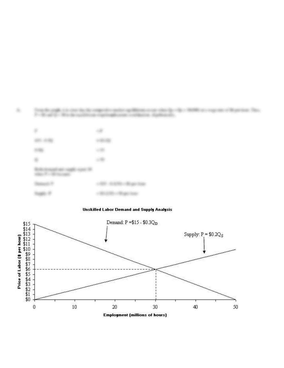
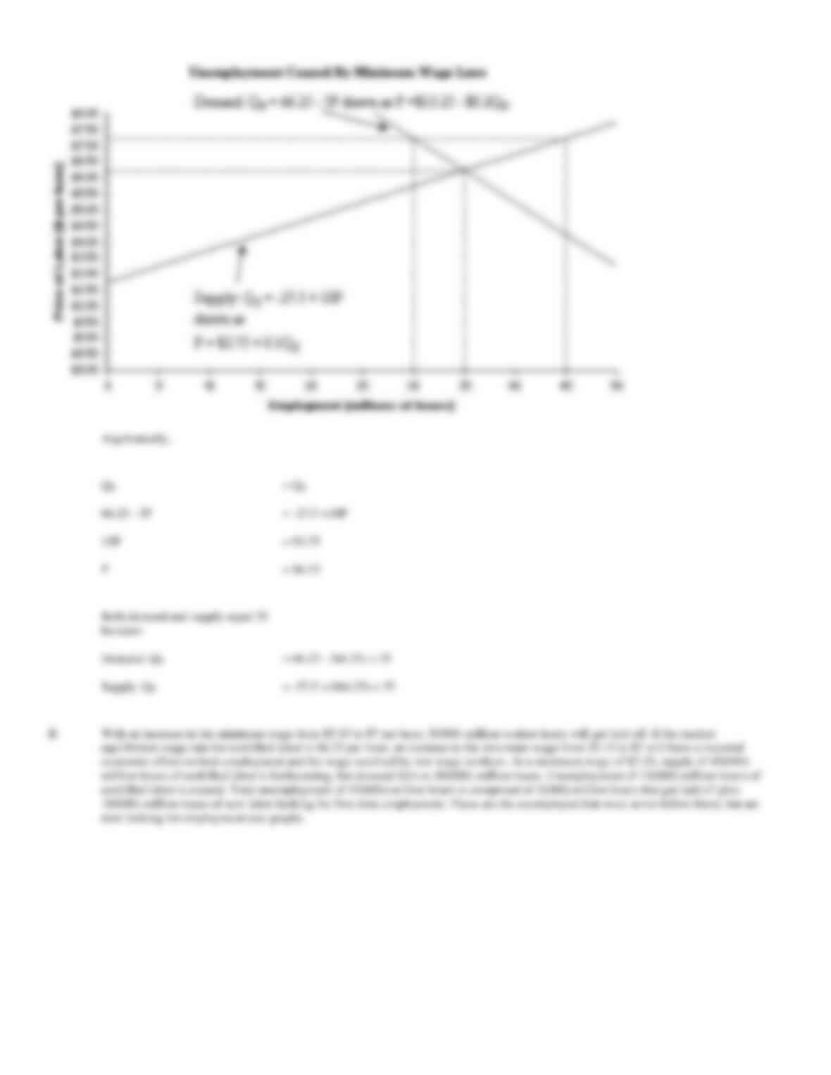
28. Competitive Market Equilibrium. Assume demand and supply conditions in the competitive market for
unskilled labor are as follows:
P
= $15 – 0.3QD
(Demand)
P
= $0.2QS
(Supply)
where Q is millions of hours of unskilled labor and P is the wage rate per hour.
A.
Illustrate the industry equilibrium wage/employment combination both graphically and algebraically.
B.
Calculate the level of excess supply (unemployment) if the Federal minimum wage is raised from $5.15 to $6 per hour.
B.
If the market equilibrium wage rate for unskilled labor is $6 per hour, an increase in the minimum wage from $5.15 to $6 will have no
economic effect. The wage rate of $6 and the equilibrium employment of 30(000) million hours will be maintained.
P
= P
$15 – 0.3Q
= $0.2Q
0.5Q
= 15
Q
= 30
Demand: P
= $15 – 0.3(30) = $6 per hour
Supply: P
= $0.2(30) = $6 per hour
29. Competitive Market Surplus. Suppose demand and supply conditions in the competitive market for
unskilled labor are as follows:
P
= $15 – 0.3QD
(Demand)
P
= $3 + $0.1QS
(Supply)
where Q is millions of hours of unskilled labor and P is the wage rate per hour.
A.
Illustrate the industry equilibrium wage/employment combination both graphically and algebraically.
B.
Calculate the level of excess supply (unemployment) if the Federal minimum wage is raised from $5.15 to $7 per hour.
Algebraically,
P
= P
$15 – 0.3Q
= $3 + $0.1Q
0.4Q
= 12
Q
= 30
Demand: P
= $15 – 0.3(30) = $6 per hour
Supply: P
= $3 + $0.1(30) = $6 per hour
30. Competitive Market Surplus. Assume demand and supply conditions in the competitive market for
unskilled labor are as follows:
QD
= 66.25 – 5P
(Demand)
QS
= -27.5 + 10P
(Supply)
where Q is millions of hours of unskilled labor and P is the wage rate per hour.
A.
Illustrate the industry equilibrium price/output combination both graphically and algebraically.
B.
How many low-wage workers will get laid off if the Federal minimum wage is raised from $5.15 to $7.25 per hour?
hours of unskilled labor is created (see graph).
31. Per Unit Tax and Elastic Demand. Assume that the supply of tickets to an outdoor music festival in
Thousand Oaks, California, is a function of price such that:
QS
= 1P
(Supply)
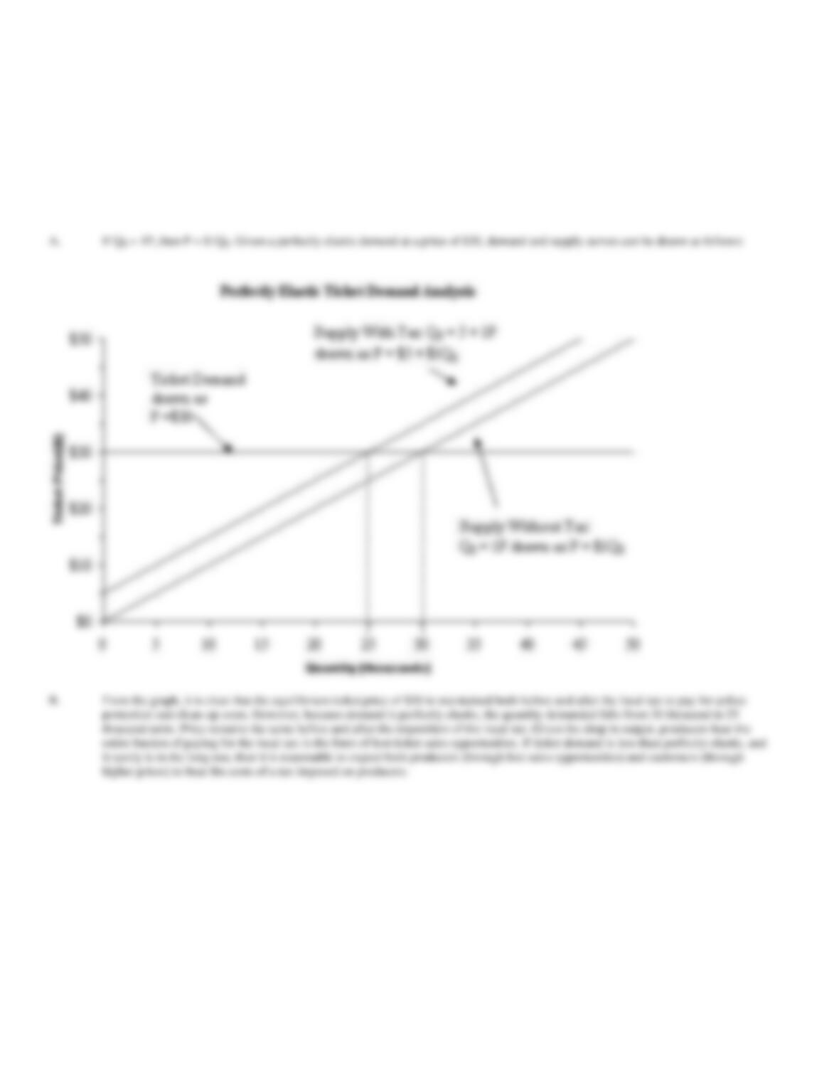
where Q is the number of tickets (in thousands) and P is the ticket price. Also assume that the demand for such concert tickets is perfectly elastic at a
price of $30. This means that the ticket demand curve can be drawn as a horizontal line that passes through $30 on the Y-axis.
A.
Graph the ticket demand and supply curves using the price of tickets as a function of quantity (Q). On this same graph, draw another
ticket supply curve based upon the assumption that a local municipality imposes a $5 tax on each ticket sold to pay for police protection
and clean-up costs.
B.
Calculate the ticket price and quantity effects of the municipal tax. With perfectly elastic demand, who pays the economic burden of
such a tax?
32. Percentage Tariff and Elastic Demand. Assume that the supply of imported personal computers (PCs)
from China is given by the expression:
QS
= 0.03125P
(Supply)
If QS = 1P, then P = $1QS. Given a perfectly elastic demand at a price of $30, demand and supply curves can be drawn as follows:
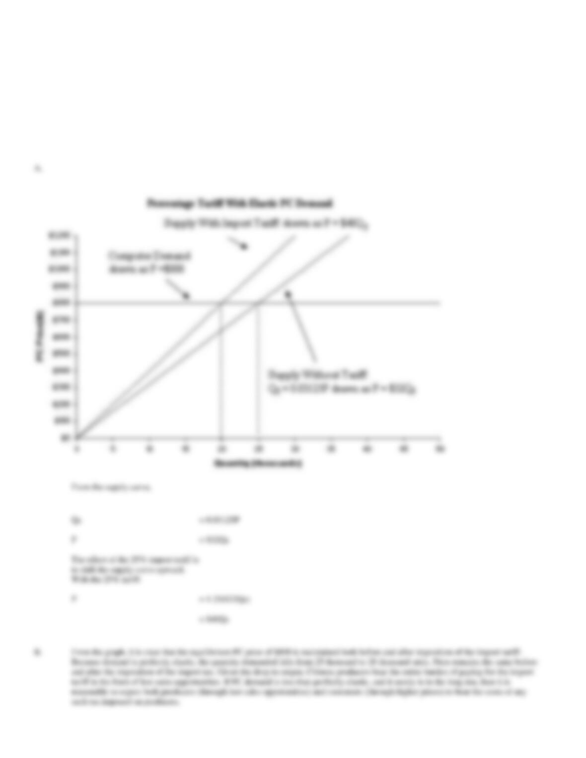
where Q is the number of PCs sold (in thousands) and P is the PC price. Given the availability of PCs on the Internet, assume that the demand for
PCs is perfectly elastic at a price of $800. This means that the PC demand curve can be drawn as a horizontal line that passes through $800 on the
Y-axis.
A.
Graph the PC demand and supply curves using price as a function of quantity (Q). On this same graph, draw another supply curve based
upon the assumption imports form China are subject to an 25% import tariff (tax) that is not imposed on imports from other countries.
B.
Calculate the PC price and quantity effects of the 25% import tariff. With perfectly elastic demand, who pays the economic burden of
such a tax?
33. Sales Tax and Elastic Demand. Assume that the supply of a best-selling book at local book stores
throughout the United States is a function price such that:
QS
= -50 + 5P
(Supply)
where Q is the number of books sold (in thousands) and P is the book price. Given the availability of this book on amazon.com for $20, demand is
perfectly elastic at a price of $20.
A.
Derive the book supply curve where price is expressed as a function of output. Calculate the equilibrium level of output and local
bookstore sales revenue.
B.
Derive a second book supply curve based upon the assumption local sales are subject to an 8% sales tax that is not imposed on Internet
sales. Calculate the book price and quantity effects of the local 8% sales tax. With perfectly elastic demand, who pays the economic
burden of such a tax?
QS
= -50 + 5P
= 50(000)
= $1,000(000)
QS
= -50 + 5P
P
= $10 + $0.2QS
is:
= $10.8 + $0.216QS
QS
= -50 + 4.63P
34. Recycling Fee and Elastic Demand. Assume that the weekly supply of 16-ounce bottles of soda at
convenience stores in the Twin Cities of Minneapolis and St. Paul is a function of price such that:
QS
= -20 + 80P
(Supply)
where Q is the number of sodas sold in convenience stores (in thousands) and P is the soda price. Assume demand is perfectly elastic at a price of $1.
A.
Derive the soda supply curve where price is expressed as a function of output. Calculate the equilibrium level of output and
convenience store sales revenue.
B.
Derive a second curve based upon the assumption convenience store sales become subject to a 5 cent recycling fee. Calculate the price
and quantity effects of the recycling fee. With perfectly elastic demand, who pays the economic burden of such a fee.
With perfectly elastic demand at a price of $1, the supply curve indicates the equilibrium level of output as:
of output as:
QS
= -50 + 4.63P
= 42.6(000)
= $852(000)
producers (through lost sales opportunities) and customers (through higher prices) to bear the costs of any such tax imposed on
producers.
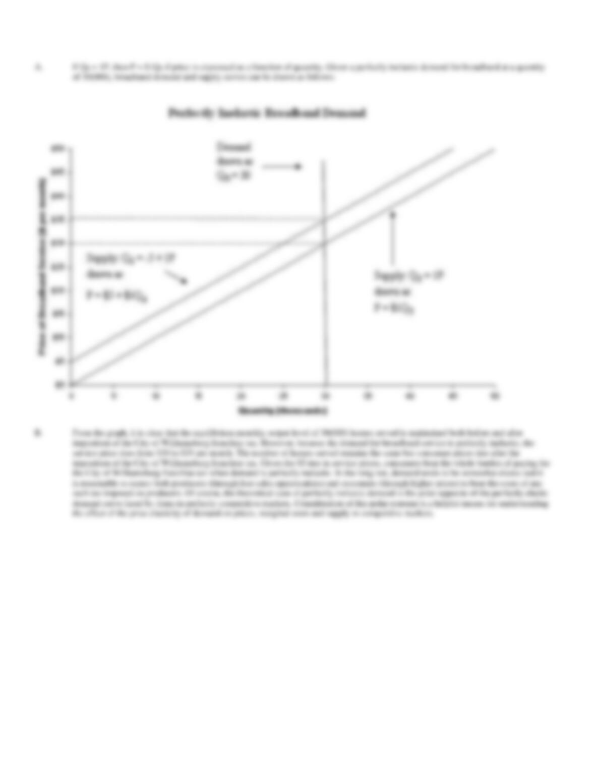
35. Franchise Tax and Inelastic Demand. Assume the supply of broadband services in the City of
Williamsburg can be described as:
QS
= 1P
(Supply)
where Q is thousands of homes served per month with broadband service, and P is the price per month. Also assume that broadband service demand
is perfectly inelastic at a quantity of 30(000). This means that the broadband demand curve can be drawn as a vertical line that passes through
30(000) on the X-axis.
A.
Graph the broadband demand and supply curves using price as a function of the quantity of service demanded (Q). On this same graph,
draw another supply curve based upon the assumption that the City of Williamsburg imposes a franchise tax that increases provider
costs by $5 per customer every month.
B.
Calculate the price and output effects of the City of Williamsburg franchise tax. With perfectly inelastic elastic demand, who pays the
costs of this tax?
QS
= 20 + QS
P
= $0.25 + $0.0125QS
P
= $0.25 + $0.0125QS + $0.05
= $0.3 + $0.0125QS
0.0125QS
QS
equilibrium level of output as:
= 56($1)
= $56(000)
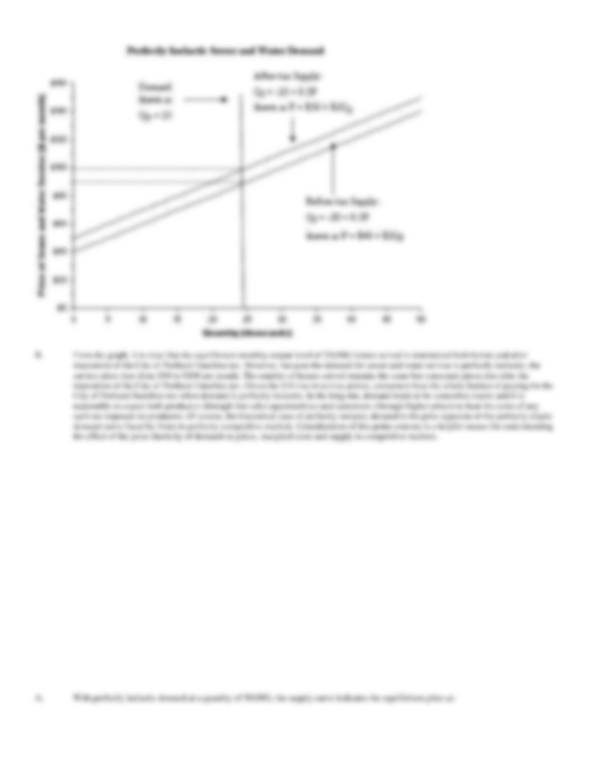
36. Franchise Tax and Inelastic Demand. Assume the supply of sewer and water services in the City of
Portland can be described as:
QS
= -20 + 0.5P
(Supply)
where Q is thousands of homes served per month with sewer and water service, and P is the price per month. Also assume that sewer and water
service demand is perfectly inelastic at a quantity of 25(000). This means that the sewer and water demand curve can be drawn as a vertical line that
passes through 25(000) on the X-axis.
A.
Graph the sewer and water demand and supply curves using price as a function of the quantity of service demanded (Q). On this same
graph, draw another supply curve based upon the assumption that the City of Portland imposes a franchise tax that increases provider
costs by $10 per customer every month.
B.
Calculate the price and output effects of the City of Portland franchise tax. With perfectly inelastic demand, who pays the costs of this
tax?
Given a perfectly inelastic demand for sewer and water at a quantity of 25(000), sewer and water demand and supply curves can be
drawn as follows:
37. Franchise Tax and Inelastic Demand. Assume the supply of sewer and water services in the City of
Greenville, North Carolina, can be described as:
QS
= -150 + 2P
(Supply)
where Q is thousands of homes served per month with sewer and water service, and P is the price per month. Also assume that sewer and water
service demand is perfectly inelastic at a quantity of 50(000).
A.
Derive the sewer and water service supply curve where price is expressed as a function of output. Calculate the equilibrium level of
output and sewer and water utility sales revenue.
B.
Derive a second sewer and water service supply curve based upon the assumption that every month the City of Greenville imposes a
$25 per customer franchise tax. Calculate the equilibrium level of output and sewer and water utility sales revenue with the tax. With
perfectly inelastic demand, who pays the economic burden of such a tax?
With perfectly inelastic demand at a quantity of 50(000), the supply curve indicates the equilibrium price as:
38. Percentage Tax and Inelastic Demand. Assume the supply of cable TV services in the City of San
Marcos, Texas, can be described as:
QS
= -5 + 0.5P
(Supply)
where Q is thousands of homes served per month with cable TV service, and P is the price per month. Also assume that cable TV service demand is
perfectly inelastic at a quantity of 25(000).
A.
Derive the cable TV service supply curve where price is expressed as a function of output. Calculate the equilibrium level of output and
cable TV utility sales revenue.
B.
Derive a second cable TV service supply curve based upon the assumption that every month the City of San Marcos imposes a 25% of
revenues franchise tax on the local cable TV company. Calculate the equilibrium level of output and cable TV sales revenue with the
tax. With perfectly inelastic demand, who pays the economic burden of such a tax?
With perfectly inelastic demand at a quantity of 25(000), the supply curve indicates the equilibrium price as:
QS
= -150 + 2P
= 150 + QS
P
= $75 + $0.5QS
= $75 + $0.5(50)
= $100
= 50($100)
= $5,000(000)
The effect of a $25 per customer franchise fee is to shift the supply curve upward in a parallel fashion. With the franchise fee:
P
= $75 + $0.5QS + $25
= $100 + $0.5(50)
= $125 (including the $25 tax)
= 50($100)
= $5,000(000)