40. Long-run Competitive Firm Supply. Calvin’s Barbershop is a popularly-priced hair cutter on the south
side of Chicago. Given the large number of competitors, the fact that barbers routinely tailor services to meet
customer needs, and the lack of entry barriers, it is reasonable to assume that the market is perfectly competitive
and that the average $15 price equals marginal revenue, P = MR = $15. Furthermore, assume that the
barbershop’s monthly operating expenses are typical of the 50 barbershops in the local market and can be
expressed by the following total and marginal cost functions:
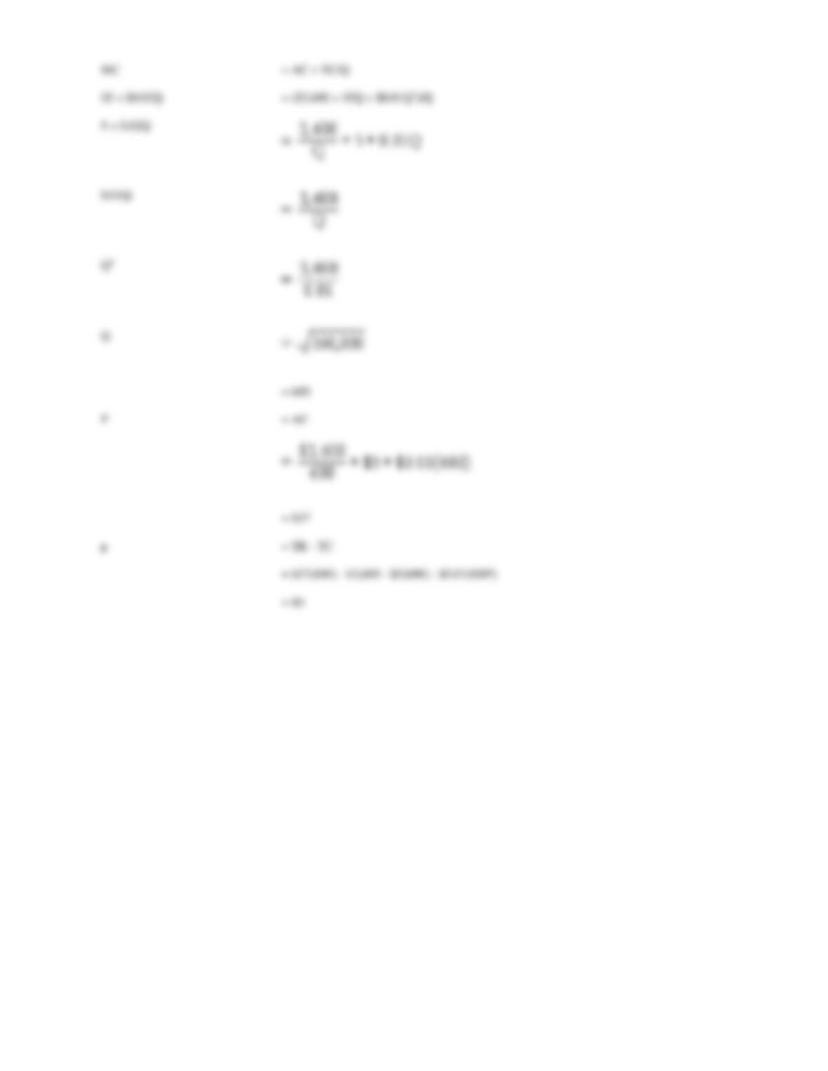
TC = $7,812.50 + $2.5Q + $0.005Q2
MC = TC/ Q = $2.5 + $0.01Q
where TC is total cost per month including capital costs, MC is marginal cost, and Q is the number of hair cuts provided. Total costs include a normal
profit.
A.
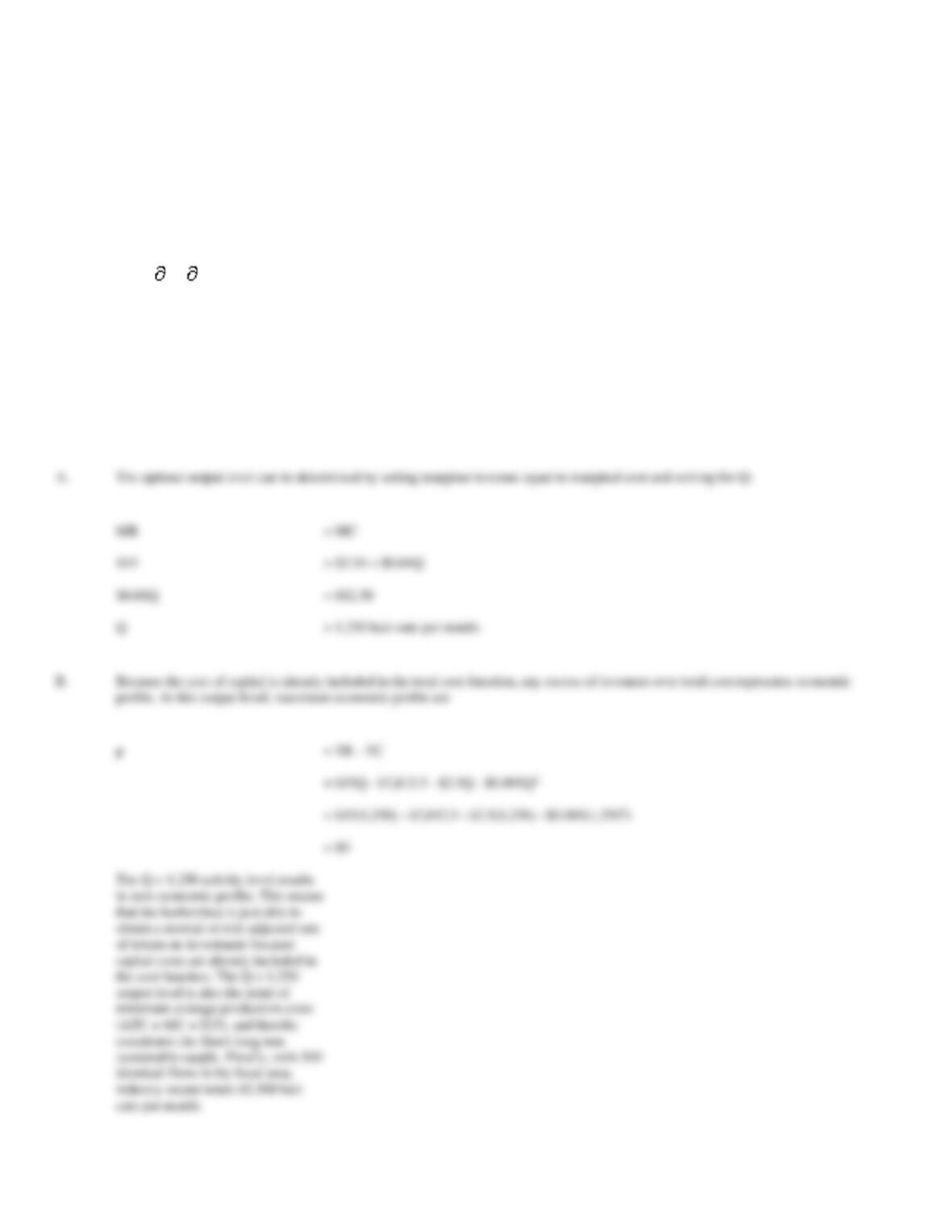
Calculate Calvin’s profit-maximizing output level.
B.
Calculate the Calvin’s economic profits at this activity level. Is this activity level sustainable in the long run?
= MC
= $12.50
Q
= 1,250 hair cuts per month.
= $15Q – $7,812.5 – $2.5Q – $0.005Q2
= $0
41. Short-run Market Supply. Carolina Textiles, Inc., is a small manufacturer of cotton linen that it sells in a
perfectly competitive market. Given $100,000 in fixed costs per day, the daily total cost function for this
product is described by:
TC = $100,000 + $2Q + $0.0625Q2
MC = TC/ Q = $2 + $0.125Q
where Q is units of cotton linen produced per day. Assume that MC > AVC at every point along the firm’s marginal cost curve, and that total costs
include a normal profit.
A.
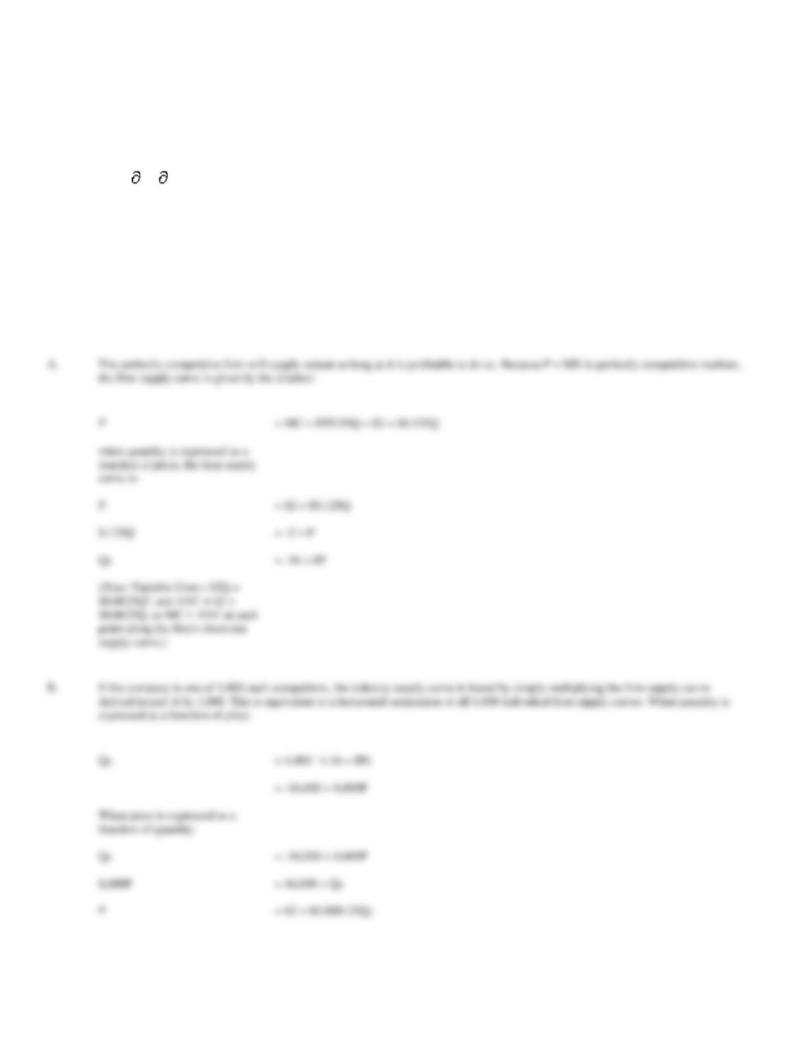
Derive the firm’s supply curve, expressing quantity as a function of price.
B.
Derive the market supply curve if North Carolina Textiles is one of 1,000 competitors.
C.
Calculate market supply per day at a market price of $47 per unit.
P
= MC = DTC/DQ = $2 + $0.125Q
P
= $2 + $0.125Q
0.125Q
= 1,000 ´ (-16 + 8P)
8,000P
= 16,000 + QS
42. Short-run Market Supply. The Fertilizer Supply Co. is a typical distributor in the perfectly competitive
fertilizer supply industry. Its marginal cost of output is:
MC = $250 + $0.05Q
where Q is tons of fertilizer produced per year.
A.
Derive the firm’s supply curve, expressing quantity as a function of price.
B.
Derive the industry supply curve if the firm is one of 400 competitors.
C.
Calculate industry supply per year at a market price of $300 per ton.
P
= MC = $250 + $0.05Q
P
= $250 + $0.05Q
0.05Q
= P – 250
= 400(-5,000 + 20P)
8,000P
= 2,000,000 + QS
P
= $250 + $0.000125QS
C.
= 360,000 units per day
43. Short-run Market Supply. Motor City Music is a local distributor of musical CDs featuring compilations
of classic rock recordings by various artists. Motor City’s marginal cost of output is described by the relation:
MC = $2.50 + $0.00025Q
where Q is CDs sold per year.
A.
Derive the firm’s supply curve, expressing quantity as a function of price.
B.
Derive the industry supply curve if the firm is one of 100 competitors.
C.
Calculate industry supply per year at a market price of $5 per unit.
P
= MC = $2.50 + $0.00025Q
P
= $2.50 + $0.00025Q
0.00025Q
= P – 2.50
C.
= 400,000
44. Short-run Market Supply. The Magazine Delivery Company is a typical firm in the perfectly competitive
magazine delivery business. The company delivers magazines and stocks magazine racks at convenience stores
located throughout the state of Kentucky. Marginal costs of service are described by the relation:
MC = $5 + $0.4Q
where Q is racks of magazines delivered and serviced per week.
A.
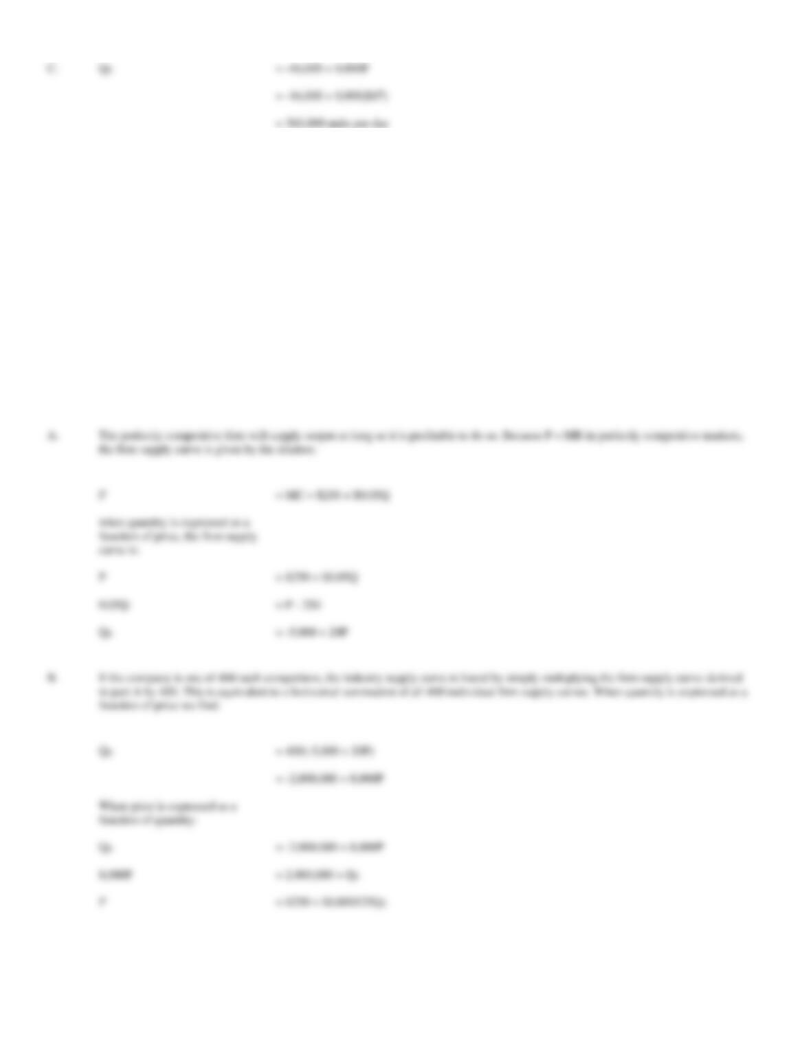
Derive the firm’s supply curve, expressing quantity as a function of price.
B.
Derive the market supply curve if the company is one of 200 competitors.
C.
Calculate market supply per week at a market price of $25 per rack delivered and serviced.
P
= MC = $5 + $0.4Q
= P – 5
= 100(-10,000 + 4,000P)
P
= $2.50 + $0.0000025QS
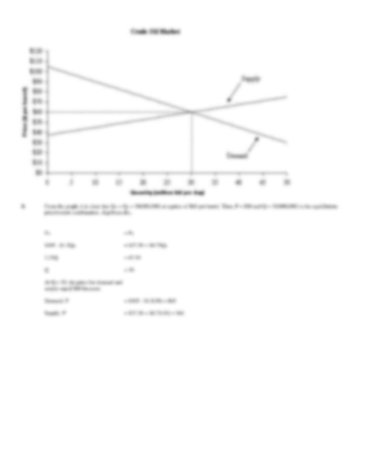
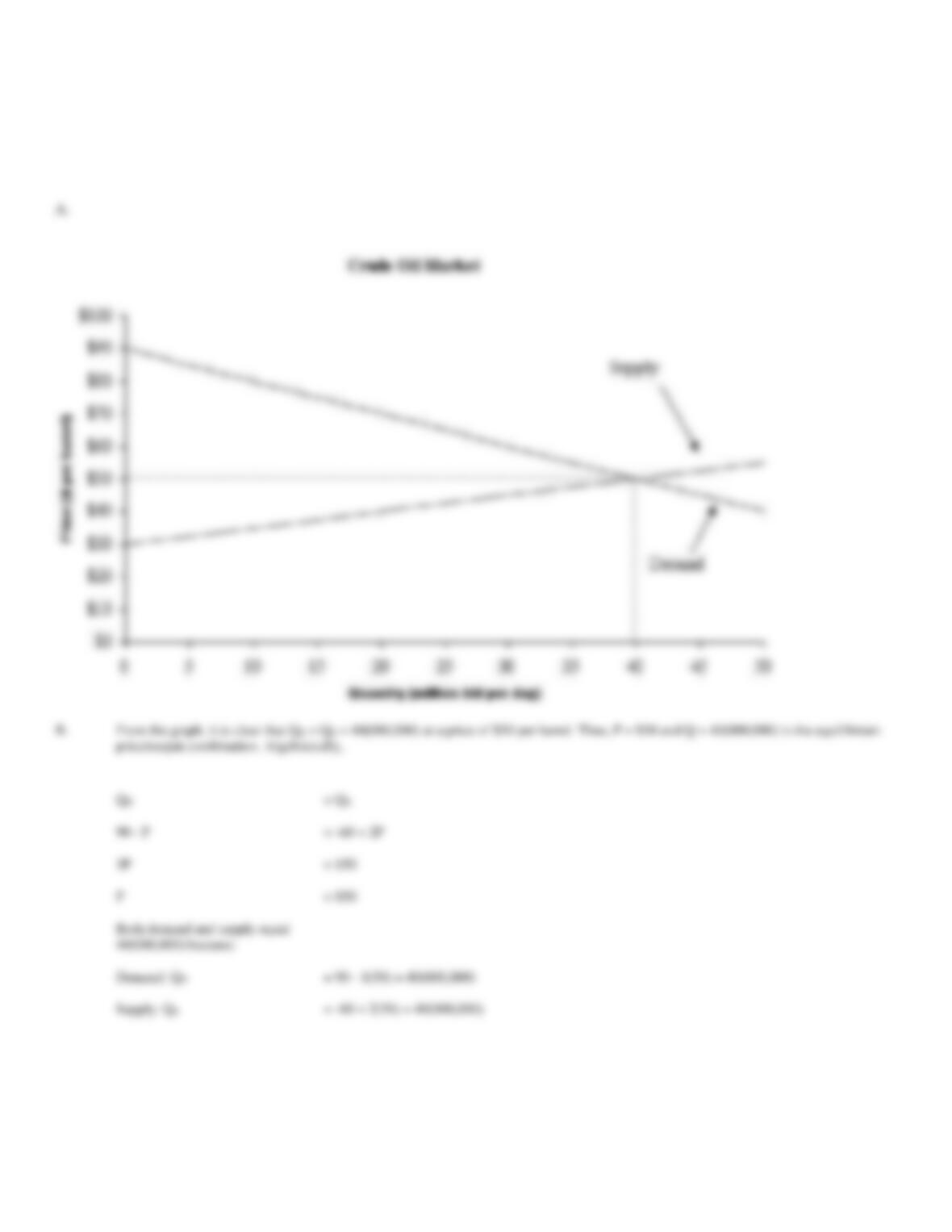
45. Perfectly Competitive Equilibrium. Fuel costs have risen sharply during recent years as consumption,
refining and production costs have increased. Demand and supply conditions in the perfectly competitive
domestic crude oil market are:
P
= $105 – 1.5QD
(Demand)
P
= $37.50+ 0.75QS
(Supply)
where P is price per barrel and Q is quantity in millions of barrels per day .
A.
Graph industry demand and supply curves.
B.
Determine both graphically and algebraically the equilibrium industry price/output combination.
A.
500P
= 2,500 + QS
P
= $5 + $0.002QS
C.
= 10,000 per week
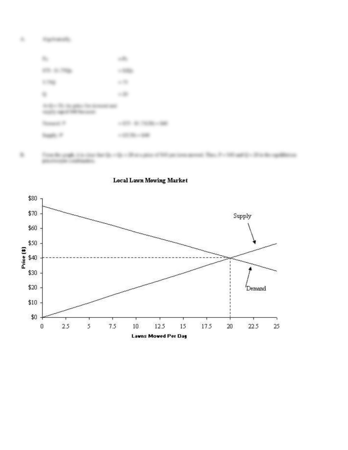
46. Perfectly Competitive Equilibrium. Lawn mowing services are supplied by a host of individuals in the
suburb of Westbrook. Demand and supply conditions in the perfectly competitive domestic for lawn mowing
services are:
P
= $75 – 1.75QD
(Demand)
P
= $2QS
(Supply)
where P is price per lawn mowed and Q is quantity of lawns mowed per day.
A.
Algebraically determine the equilibrium industry price/output combination.
B.
Confirm this by graphing industry demand and supply curves.
= PS
$105 – $1.5QD
= $37.50 + $0.75QS
2.25Q
= 67.50
Q
= 30
Demand: P
= $105 – $1.5(30) = $60
Supply: P
= $37.50 + $0.75(30) = $60
47. Perfectly Competitive Equilibrium. Fuel costs have risen quickly during recent years as consumption,
refining and production costs have risen sharply. Supply and demand conditions in the perfectly competitive
domestic crude oil market are:
QS
= -60 + 2P
(Supply)
QD
= 90 – P
(Demand)
Algebraically,
$75 – $1.75QD
= $2QS
Q
= 20
Demand: P
= $75 – $1.75(20) = $40
Supply: P
= $2(20) = $40
where Q is quantity in millions of barrels per day, and P is price per barrel.
A.
Graph industry supply and demand curves.
B.
Determine both graphically and algebraically the equilibrium industry price/output combination.
A.
P
= $50
Demand: QD
= 90 – 1(50) = 40(000,000)
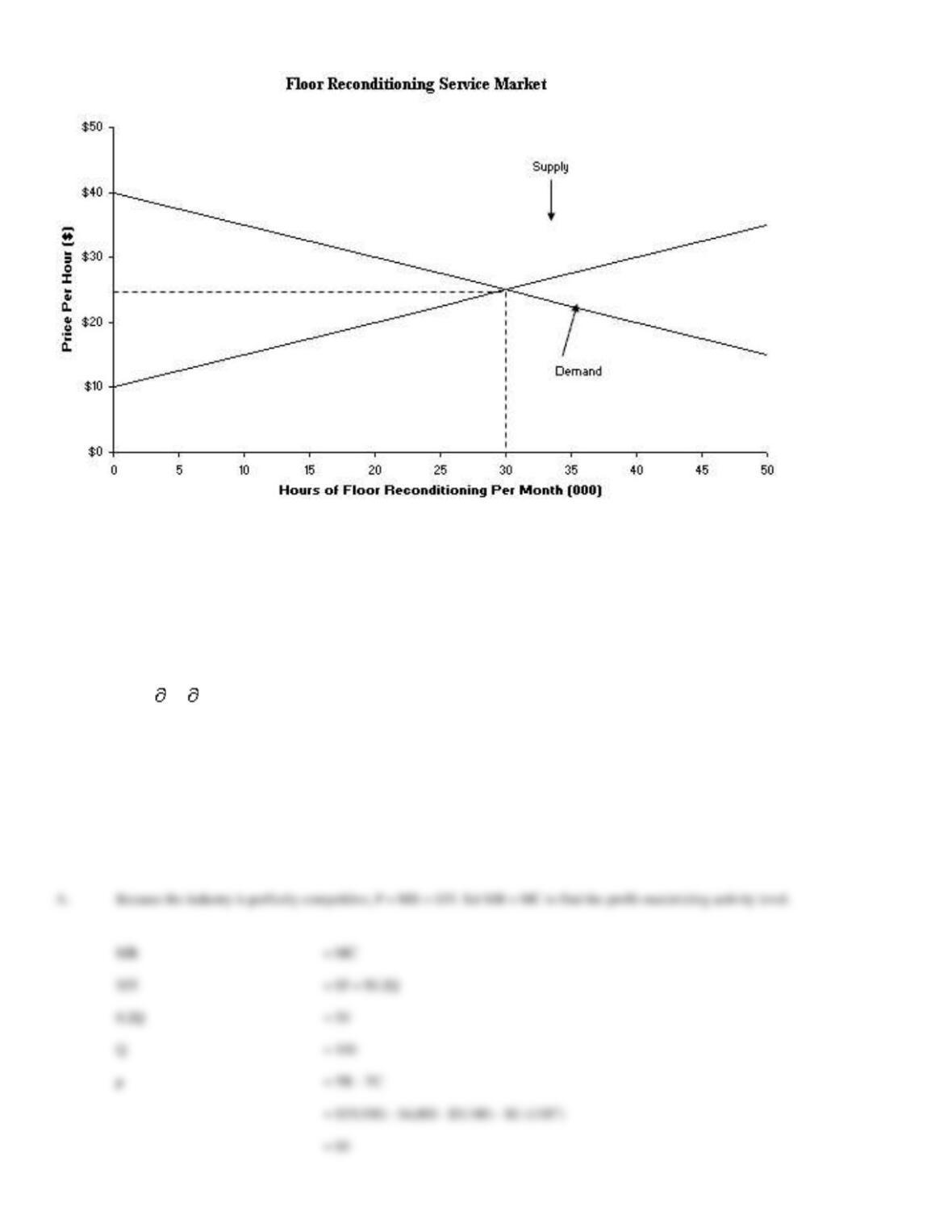
48. Perfectly Competitive Equilibrium. Office building maintenance plans call for the stripping, waxing, and
buffing of ceramic floor tiles. This work is often contracted out to office maintenance firms, and both
technology and labor requirements are very basic. Supply and demand conditions in this perfectly competitive
service market in St. Paul, Minnesota, are:
QS
= -20 + 2P
(Supply)
QD
= 80 – 2P
(Demand)
where Q is thousands of hours of floor reconditioning per month, and P is the price per hour.
A.
Algebraically determine the market equilibrium price/output combination.
B.
Use a graph to confirm your answer.
Algebraically,
QD
= QS
= -20 + 2P
= 100
P
= $25 per hour
Demand:
QD = 80 – 2($25) = 30(000)
Supply:
QS = -20 + 2($25) = 30(000)
49. Competitive Market Equilibrium. Happy Valley Supply, Inc., provides recycled toner cartridges for
printers. Like its competitors, Happy Valley must meet strict specifications. As a result, the replacement toner
cartridge market can be regarded as perfectly competitive. Total and marginal cost relations per week are:
TC = $4,000 + $5Q + $0.1Q2
MC = TC/ Q = $5 + $0.2Q
where Q is the number of recycled toner cartridges.
A.
Calculate Happy Valley’s optimal output and profits if prices are stable at $55 per toner cartridge.
B.
Calculate Happy Valley’s optimal output and profits if prices rise to $65 per unit.
C.
If Happy Valley is typical of firms in the industry, calculate the firm‘s equilibrium output, price, and profit levels.
A.
Because the industry is perfectly competitive, P = MR = $55. Set MR = MC to find the profit-maximizing activity level.
= MC
= $5 + $0.2Q
0.2Q
= 50
Q
= 100
50. Competitive Market Equilibrium. Syracuse Paper supplies printer paper in upstate New York. Like the
output of other wholesale distributors, Syracuse Paper must meet strict guidelines and the printer paper supply
industry can be regarded as perfectly competitive. Total and marginal cost relations are:
TC = $3,600 + $5Q + $0.01Q2
MC = TC/ Q = $5 + $0.02Q
where Q is cases of printer paper per day.
A.
Calculate the firm’s optimal output and profits if prices are stable at $20 per case.
B.
Calculate optimal output and profits if prices rise to $25 per case.
C.
If Syracuse Paper is typical of firms in the industry, calculate the firm‘s equilibrium output, price, and profit levels.
= MC
0.02Q
= 15
p
= TR – TC
= $20(750) – $3,600 – $5(750) – $0.01(7502)
= $2,025
B.
After a rise in prices to $25, the optimal activity level grows to Q = 1,000 because:
= MC
= $5 + $0.02Q
0.02Q
= 20
Q
= 1,000
p
= TR – TC
= $25(1,000) – $3,600 – $5(1,000) – $0.01(1,0002)
= $6,400
C.
In equilibrium, P = AC and MR = MC at the point where average cost is minimized. To find the point of minimum average costs set: