1. In macroeconomics, equilibrium is defined as the point at which:
a.
the economy attains the highest level of GDP.
b.
there is no unemployment in the economy.
c.
people’s plans match the reality.
d.
there is high inflation and unemployment in the economy.
e.
there is no inflation in the economy.
2. The equilibrium level of income will rise when:
a.
planned consumption spending is less than real GDP.
b.
taxes exceed saving.
c.
supply exceeds demand.
d.
planned inventory investment is negative.
e.
aggregate expenditures exceed real GDP.
MACR.BOYE.16.48 – ch. 10, 2
Equilibrium Income and Expenditures
3. If aggregate expenditures are less than real GDP, then:
a.
both inventories and real GDP will decline.
b.
inventories will decline but real GDP will increase.
c.
inventories will increase and real GDP will decline.
d.
both inventories and real GDP will increase.
e.
inventories will increase but real GDP will remain unchanged.
MACR.BOYE.16.48 – ch. 10, 2
United States – Equilibrium
Equilibrium Income and Expenditures
4. Which of the following is true at the equilibrium level of income?
a.
Unplanned inventory changes are positive.
b.
Firms are unable to produce the desired rate of output.
MACR.BOYE.16.47 – ch. 10, 1
Equilibrium Income and Expenditures
c.
Autonomous consumption spending is equal to induced consumption spending.
d.
Aggregate expenditures equal real GDP.
e.
Unplanned investment spending is positive.
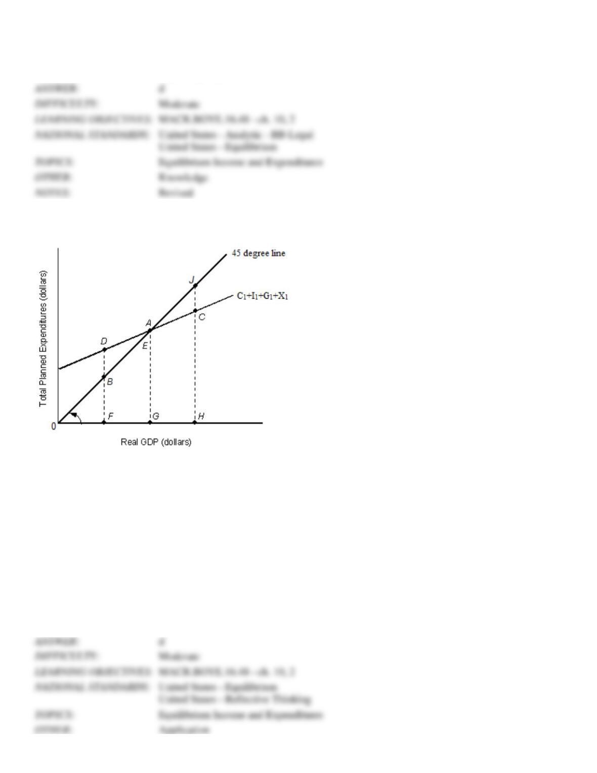
The figure given below shows the aggregate expenditure curve of an open economy.
Figure 10.1
In the figure:
C1: Consumption
I1: Investment
G1: Government spending
X1: Net Exports
5. Consider the economy described in Figure 10.1. Which of the following is true if the real GDP is equal to 0H?
a.
Aggregate expenditures are greater than total income, when the real GDP is equal to OH.
b.
All economic resources are being used efficiently, when the real GDP is equal to OH.
c.
Households are dissaving an amount equal to DC, when the real GDP is equal to OH.
d.
Businesses accumulate unwanted inventories, when the real GDP is equal to OH.
e.
Unplanned investment decline, when the real GDP is equal to OH.
MACR.BOYE.16.48 – ch. 10, 2
Equilibrium Income and Expenditures
MACR.BOYE.16.48 – ch. 10, 2
United States – Equilibrium
Equilibrium Income and Expenditures
6. According to Figure 10.1, when real GDP is at G:
a.
there is pressure for the economy to expand.
b.
there are unplanned reductions in inventory.
c.
aggregate expenditures are less than real GDP.
d.
the economy is at the macroeconomic equilibrium.
e.
there is pressure for the economy to contract.
d
Moderate
MACR.BOYE.16.48 – ch. 10, 2
United States – Reflective Thinking
Equilibrium Income and Expenditures
Application
7. According to Figure 10.1, the economy will expand when aggregate expenditures are at:
a.
point D.
b.
point A.
c.
point B.
d.
point C.
e.
point E.
Moderate
MACR.BOYE.16.48 – ch. 10, 2
Equilibrium Income and Expenditures
Application
The table given below states the value of the GDP and the different components of aggregate expenditure for two years.
Table 10.1
GDP
Export
Import
Year 1
—
$750
$110
$60
$70
$50
Year 2
$1,150
$930
$90
$75
$125
—
8. Refer to Table 10.1. What is the equilibrium level of real GDP in year 1?
a.
$940
b.
$1,040
c.
$1,100
d.
$1,050
e.
$920
Moderate
MACR.BOYE.16.48 – ch. 10, 2
United States – Reflective Thinking
Revised
9. Refer to Table 10.1. Assume that the economy is at equilibrium in both years. What are net exports for year 2?
a.
$60
b.
$125
c.
$70
d.
$55
e.
$195
d
Moderate
MACR.BOYE.16.48 – ch. 10, 2
United States – Reflective Thinking
Equilibrium Income and Expenditures
Application
10. Refer to Table 10.1. If real GDP equals $1,000 in year 1, then:
a.
unplanned inventory investment is zero.
b.
unplanned inventories increase by $50.
c.
inventories decrease by $100.
d.
inventories increase by $60.
e.
real GDP is less than aggregate expenditure.
d
Moderate
MACR.BOYE.16.48 – ch. 10, 2
United States – Reflective Thinking
Equilibrium Income and Expenditures
Application
11. Refer to Table 10.1. What would be the new equilibrium level of real GDP in year 2 if net exports equaled zero?
a.
$1,205
b.
$1,095
c.
$1,050
d.
$1,170
e.
$1,120
b
Challenging
MACR.BOYE.16.48 – ch. 10, 2
Equilibrium Income and Expenditures
Application
12. Refer to Table 10.1. What is the level of imports in year 2, if the economy is in equilibrium?
Equilibrium Income and Expenditures
Application
a.
$20
b.
$50
c.
$70
d.
$100
e.
$120
13. Assume we are at an income level where the C+I+G+X (consumption+investment+government spending+net exports)
function lies above the 45-degree line. We can conclude that at this income level:
a.
unplanned inventories are likely to accumulate.
b.
the economy is in equilibrium.
c.
households will save more money than they spend.
d.
aggregate expenditures are less than output.
e.
there will be pressure to expand production.
Moderate
MACR.BOYE.16.48 – ch. 10, 2
Equilibrium Income and Expenditures
Knowledge
The table given below shows the levels of national income (Y) and the corresponding levels of saving (S), investment (I),
export (X), and import (M) of an open economy.
Table 10.2
Y
S
I
G
X
M
$935
−$250
$320
$40
$170
$100
$2,100
$0
$320
$140
$170
$130
$3,320
$250
$320
$200
$200
$350
$4,800
$375
$320
$240
$230
$415
$5,230
$650
$320
$320
$250
$590
$6,300
$825
$320
$340
$270
$610
Taxes equal zero
14. Consider the economy described in Table 10.2. What is the equilibrium level of real GDP?
a.
$935
b.
$2,100
c.
$3,320
d.
$4,800
e.
$5,230
d
Moderate
MACR.BOYE.16.48 – ch. 10, 2
United States – Reflective Thinking
Equilibrium Income and Expenditures
Application
Revised
15. Consider the economy described in Table 10.2. Calculate the level of consumption spending when the economy is in
equilibrium.
a.
$4,425
b.
$4,010
c.
$4,050
d.
$5,175
e.
$4,800
Moderate
MACR.BOYE.16.48 – ch. 10, 2
Equilibrium Income and Expenditures
Application
16. Consider the economy described in Table 10.2. Calculate the value of leakages from the economy when the economy
is in equilibrium.
a.
$770
b.
$720
c.
$790
d.
$600
e.
$410
Moderate
MACR.BOYE.16.49 – ch. 10, 3
Equilibrium Income and Expenditures
17. Consider the economy described in Table 10.2. At an income level of $2,100:
a.
leakages exceed injections by $800.
b.
total output exceeds aggregate expenditures by $500.
c.
injections exceed leakages by $500.
d.
injections are equal to total output.
e.
aggregate expenditures exceed total output by $500.
Moderate
United States – Equilibrium
Moderate
MACR.BOYE.16.48 – ch. 10, 2
Equilibrium Income and Expenditures
Application
18. Consider the economy described in Table 10.2. If autonomous saving decreases by $200, what will happen at the
current equilibrium level of income?
a.
Autonomous consumption spending will also decrease by $200, and so no change in equilibrium income
occurs.
b.
Total leakages in the economy will exceed total injections.
c.
There will be pressure on real GDP to rise.
d.
There will be pressure on the economy to contract.
e.
Unplanned inventories in the economy will grow.
MACR.BOYE.16.49 – ch. 10, 3
United States – Equilibrium
Equilibrium Income and Expenditures
Application
19. Which of the following can be considered an injection into an economy?
a.
Imports
b.
Investment
c.
Aid to foreign countries
d.
Saving
e.
Taxes
b
Easy
MACR.BOYE.16.49 – ch. 10, 3
United States – Analytic – BB-Legal
United States – Equilibrium
Equilibrium Income and Expenditures
Knowledge
Revised
20. Assume that an economy is in equilibrium with a budget deficit of $130 billion, positive net exports of $453 billion,
and savings equal to $1,550 billion. If taxes are zero, then planned investment spending must be equal to:
a.
$1,550 billion.
b.
$130 billion.
c.
$1,873 billion.
d.
$1,227 billion.
e.
$967 billion.
Challenging
MACR.BOYE.16.49 – ch. 10, 3
United States – Reflective Thinking
Equilibrium Income and Expenditures
Application
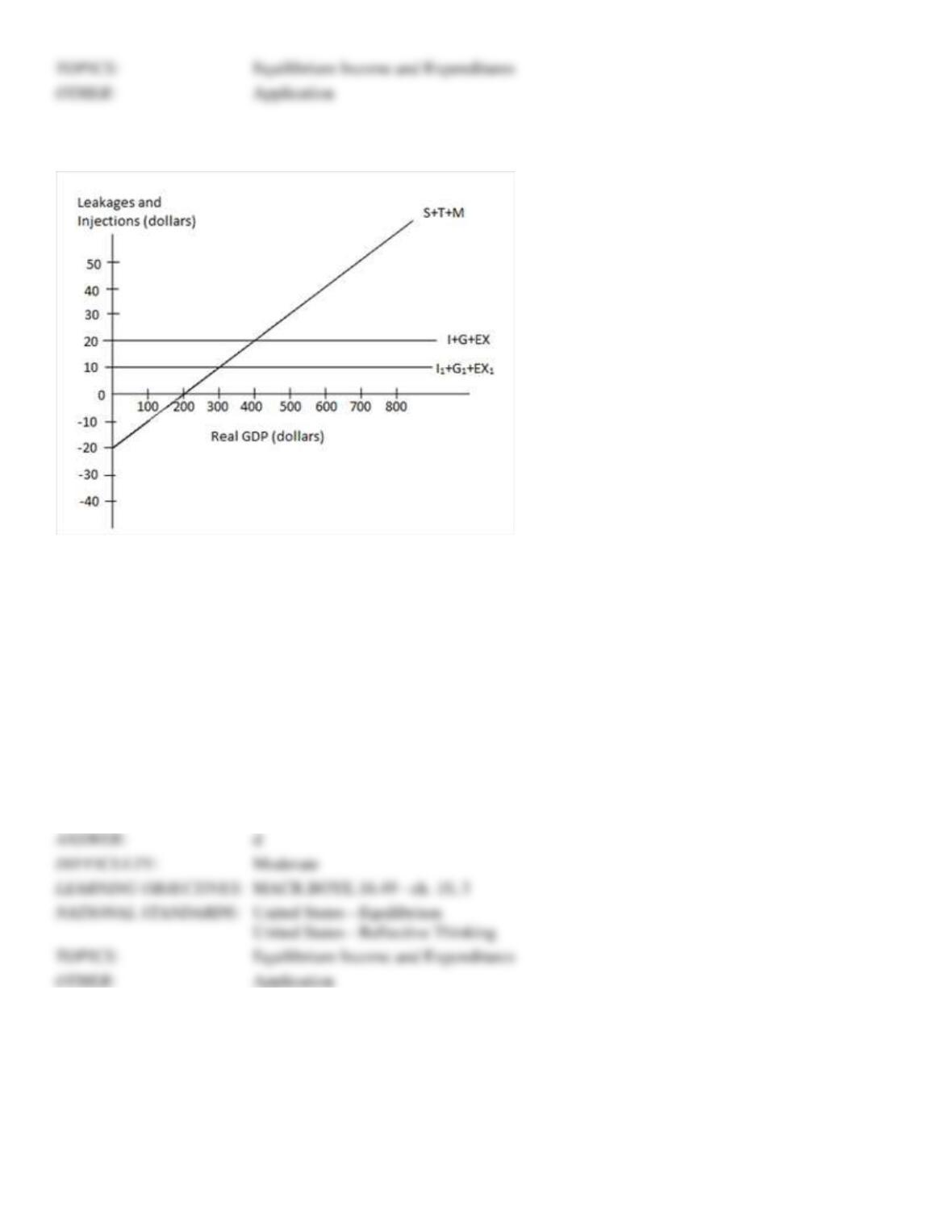
The figure given below represents the leakages and injections in an economy.
Figure 10.2
In the figure:
I, I1: Investment;
G: Government spending;
EX, EX1: Exports;
T: Taxes; and
M: Imports.
21. Refer to Figure 10.2. When total injections equal $20, the equilibrium level of real GDP is:
a.
$100.
b.
$200.
c.
$300.
d.
$400.
e.
$500.
d
Moderate
MACR.BOYE.16.49 – ch. 10, 3
Equilibrium Income and Expenditures
Application
22. Refer to Figure 10.2. A decline in total injections, from $20 to $10:
a.
will cause equilibrium income to rise to $400.
b.
will result in a disequilibrium of $200 in the economy.
c.
will cause the total leakages curve to shift inward.
d.
will cause equilibrium income to fall to $300.
e.
will not affect equilibrium income.
Equilibrium Income and Expenditures
Application
23. Refer to Figure 10.2. Suppose that I+G+EX equals $20 and the economy is in equilibrium. What is the amount of
saving when T = $0 and M = $5 at the equilibrium level?
a.
$0
b.
$10
c.
$15
d.
$20
e.
$25
Moderate
MACR.BOYE.16.49 – ch. 10, 3
United States – Reflective Thinking
Equilibrium Income and Expenditures
Application
24. According to Figure 10.2, real GDP of $200 indicates a point where:
a.
total leakages exceed total injections.
b.
aggregate expenditures exceed total output.
c.
consumers engage in dissaving.
d.
the economy is in macroeconomic equilibrium.
e.
unplanned inventory changes will be positive.
b
Challenging
MACR.BOYE.16.49 – ch. 10, 3
United States – Reflective Thinking
Equilibrium Income and Expenditures
Application
25. Savings are good for a family. If all families increase savings, the economy is better off. This fallacy of composition is
called:
a.
the paradox of time.
b.
the paradox of dissaving.
c.
the paradox of thrift.
d.
the paradox of value.
e.
the paradox of choice.
Moderate
d
Moderate
MACR.BOYE.16.49 – ch. 10, 3
United States – Reflective Thinking
Equilibrium Income and Expenditures
Application
Revised
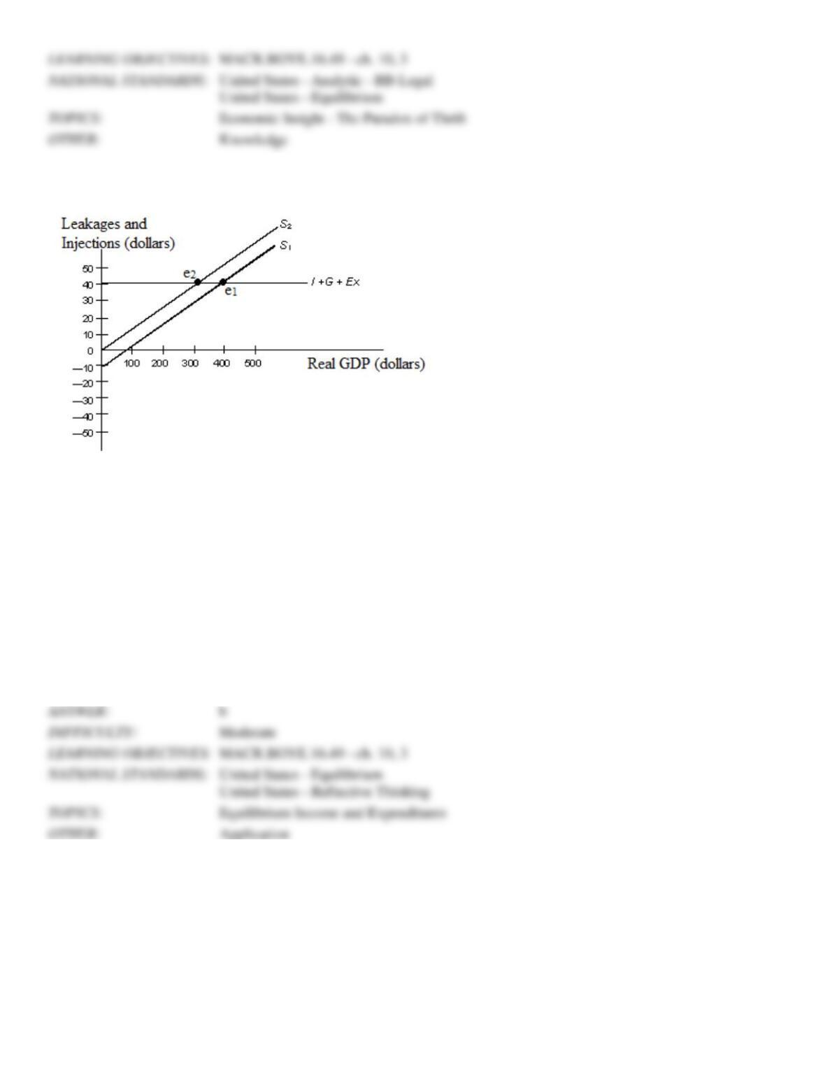
The figure given below represents the leakages and injections in an economy.
Figure 10.3
In the figure:
S1 and S2: Saving functions
I: Investment
G: Government spending
EX: Net exports
26. Refer to Figure 10.3. If saving is represented by S1, at a real GDP level of $500:
a.
leakages are greater than injections which will cause income to increase.
b.
leakages are greater than injections which will cause income to decrease.
c.
leakages are less than injections which will cause income to increase.
d.
leakages are less than injections which will cause income to decrease.
e.
leakages are equal to injections which will cause no change in income.
MACR.BOYE.16.49 – ch. 10, 3
United States – Reflective Thinking
Equilibrium Income and Expenditures
27. In Figure 10.3, which of the following represents the paradox of thrift?
a.
A shift of the saving curve from S2 to S1
b.
A shift of the saving curve from S1 to S2
c.
A change in equilibrium real GDP from $100 to $200
d.
A change in equilibrium real GDP from $300 to $100
e.
A change in equilibrium real GDP from $100 to $400
MACR.BOYE.16.49 – ch. 10, 3
Economic Insight – The Paradox of Thrift
28. Refer to Figure 10.3. The paradox of thrift might not be a problem if:
a.
the average price level does not change in the short run.
b.
the I + G + EX line were downward-sloping.
c.
the I + G + EX line were constant at an intercept of $30.
d.
the increase in saving was used to fund investment expenditures.
e.
the I + G + EX line were constant at an intercept of $50.
d
DIFFICULTY:
Challenging
MACR.BOYE.16.49 – ch. 10, 3
United States – Reflective Thinking
Equilibrium Income and Expenditures
OTHER:
Application
29. If Saving+Tax+Import > Investment+Government spending+Export, then _____ must fall to establish macroeconomic
equilibrium.
a.
net exports
b.
gross exports
c.
taxes
d.
real GDP
e.
government spending
d
DIFFICULTY:
Challenging
MACR.BOYE.16.49 – ch. 10, 3
United States – Reflective Thinking
Equilibrium Income and Expenditures
OTHER:
Comprehension
Revised
30. Suppose in an economy, investment = $40, saving = $50, government spending+export = $100 and taxes+imports =
$110. Then for this economy, total leakages exceed total injections by:
a.
$30.
b.
$25.
c.
$10.
d.
$45.
e.
$20.
ANSWER:
e
ANSWER:
b
DIFFICULTY:
Moderate
MACR.BOYE.16.49 – ch. 10, 3
United States – Reflective Thinking
TOPICS:
Equilibrium Income and Expenditures
OTHER:
Application
Revised
31. Suppose an economy operates at a real GDP level of $855, where saving = $400; investment = $95; government
spending = $365; taxes = $130; imports = $210; exports = $170. Which of the following statements is true in the light of
the given information?
a.
Aggregate expenditures will fall, because total injections exceed total leakages by $110.
b.
Real GDP will increase, because total injections are less than $855.
c.
The economy will be in equilibrium, because leakages equal injections.
d.
Real GDP will fall, because total leakages exceed total injections by $110.
e.
Inventories will rise, because planned saving exceeds planned investment.
d
Moderate
MACR.BOYE.16.49 – ch. 10, 3
United States – Reflective Thinking
Equilibrium Income and Expenditures
Application
32. Suppose an economy has a government budget surplus of $100, net exports of -$400, and a planned investment level
of $1,000. For this economy to be in equilibrium, saving must equal:
a.
$700.
b.
$500.
c.
$750.
d.
$250.
e.
$300.
Challenging
MACR.BOYE.16.49 – ch. 10, 3
United States – Reflective Thinking
Equilibrium Income and Expenditures
Application
Revised
33. Ceteris paribus, a downward shift in the net exports function will cause:
a.
equilibrium real GDP to decrease.
b.
equilibrium real GDP to increase.
c.
savings to decrease.
d.
net exports to increase.
e.
government budget deficit to decline.
Moderate
MACR.BOYE.16.49 – ch. 10, 3
Equilibrium Income and Expenditures
Application
34. The percentage of a change in income that is spent domestically is:
a.
the sum of the MPC and the MPI.
b.
the sum of the MPC and the MPS.
c.
the difference between the MPC and the MPI.
d.
the product of the MPC and the MPI.
e.
the sum of the MPS and the MPI.
Easy
MACR.BOYE.16.50 – ch. 10, 4
Changes in Equilibrium Income and Expenditures
Knowledge
Revised
35. The spending multiplier measures the change in equilibrium income that results from a change in:
a.
consumption.
b.
interest rates.
c.
savings.
d.
net exports.
e.
autonomous expenditures.
Easy
MACR.BOYE.16.51 – ch. 10, 5
Changes in Equilibrium Income and Expenditures
Knowledge
Revised
36. At each round of the multiplier process, increases in income:
a.
leak out of the expenditures stream in the form of investment and taxes.
b.
leak out of the expenditures stream in the form of saving and imports.
c.
are matched by a smaller increase in expenditures.
d.
result in even greater increases in expenditures due to investment and exports.
e.
result in no change in total expenditures.
Easy
MACR.BOYE.16.51 – ch. 10, 5
MACR.BOYE.16.49 – ch. 10, 3
Equilibrium Income and Expenditures
Comprehension
37. Assume that the marginal propensity to consume equals 0.75 and the marginal propensity to import equals 0.10. By
how much does spending on domestic goods increase if income increases by $300?
a.
$195
b.
$225
c.
$30
d.
$300
e.
$75
Challenging
MACR.BOYE.16.51 – ch. 10, 5
United States – Equilibrium
United States – Reflective Thinking
Changes in Equilibrium Income and Expenditures
Application
38. Assume that an increase of $300 in exports leads to an increase of $750 in equilibrium income. If the marginal
propensity to import equals 1/10, the marginal propensity to save must be _____.
a.
0.60
b.
0.50
c.
0.40
d.
0.30
e.
0.25
d
Challenging
MACR.BOYE.16.51 – ch. 10, 5
United States – Equilibrium
United States – Reflective Thinking
Changes in Equilibrium Income and Expenditures
Application
Scenario 10.1
Imagine an economy that does not have international trade and is initially in equilibrium. Later the government increases
the level of spending by $350 million because it received a gift from abroad. In this economy, only 65 cents of every
dollar is spent, and the rest is saved.
39. Refer to Scenario 10.1. What is the marginal propensity to save for this economy?
a.
0.5
b.
0.25
c.
0.65
d.
0.35
e.
Cannot be determined
d
United States – Equilibrium
Changes in Equilibrium Income and Expenditures
Knowledge
40. What is the marginal propensity to consume for the economy described in Scenario 10.1?
a.
0.45
b.
0.85
c.
0.65
d.
0.35
e.
Cannot be determined
Moderate
MACR.BOYE.16.51 – ch. 10, 5
Changes in Equilibrium Income and Expenditures
Application
41. Refer to Scenario 10.1. Calculate the value of the spending multiplier for this economy.
a.
2.86
b.
0.286
c.
1.54
d.
0.154
e.
0.35
Moderate
MACR.BOYE.16.51 – ch. 10, 5
United States – Reflective Thinking
Changes in Equilibrium Income and Expenditures
Application
42. Refer to Scenario 10.1. The new equilibrium level of GDP for the economy will be higher by approximately:
a.
$1 billion.
b.
$350 million.
c.
$65 million.
d.
$227.5 million.
e.
$227.5 million.
Moderate
MACR.BOYE.16.51 – ch. 10, 5
United States – Reflective Thinking
MACR.BOYE.16.51 – ch. 10, 5
Changes in Equilibrium Income and Expenditures
Application
Scenario 10.2
A hypothetical open economy has a marginal propensity to import (MPI) equal to 0.2 and a marginal propensity to
consume equal to 0.7. Assume that the economy is initially in equilibrium.
43. Refer to Scenario 10.2. What is the marginal propensity to save of this economy?
a.
0.2
b.
0.3
c.
0.7
d.
0.9
e.
0.6
b
Easy
MACR.BOYE.16.51 – ch. 10, 5
United States – Equilibrium
Changes in Equilibrium Income and Expenditures
Application
44. Refer to Scenario 10.2. What is the spending multiplier of this economy?
a.
2
b.
1.4
c.
0.7
d.
0.9
e.
Cannot be determined with the given information
Moderate
MACR.BOYE.16.51 – ch. 10, 5
United States – Equilibrium
United States – Reflective Thinking
Changes in Equilibrium Income and Expenditures
Application
45. Refer to Scenario 10.2. What will happen to the equilibrium real GDP if a tourist visits the country and spends $100
that she brought with her?
a.
It will not change.
b.
It will increase by $100.
c.
It will increase by $200.
d.
It will increase by $143.
e.
It will increase by $90.
Moderate
MACR.BOYE.16.51 – ch. 10, 5
Application
Revised
46. If MPS is equal to 0.15 and MPI is equal to 0.10, an initial change of $19,000 in government expenditure would result
in a total change of _____ in income.
a.
$19,000
b.
$16,150
c.
$20,000
d.
$76,000
e.
$126,667
d
Challenging
MACR.BOYE.16.51 – ch. 10, 5
United States – Reflective Thinking
Changes in Equilibrium Income and Expenditures
Application
Revised
47. What is the value of the spending multiplier when MPC = 0.85 and MPI = 0.3?
a.
1.82
b.
0.85
c.
2.22
d.
1.18
e.
2.50
Moderate
MACR.BOYE.16.51 – ch. 10, 5
United States – Reflective Thinking
Changes in Equilibrium Income and Expenditures
Application
48. Consider an economy that is in equilibrium with real GDP = $5,000, MPS = 1/4 and MPI = 1/5. What will be the new
equilibrium level of income if planned investment spending increases by $500?
a.
$15,000
b.
$7,000
c.
$6,111
d.
$5,500
e.
$5,000
MACR.BOYE.16.51 – ch. 10, 5
Changes in Equilibrium Income and Expenditures
Changes in Equilibrium Income and Expenditures
Knowledge
Revised
49. If equilibrium income is $500 billion, MPC = 0.8, MPI = 0.2 and autonomous government spending increases by $20
billion, the new equilibrium income will be _____.
a.
$600 billion
b.
$550 billion
c.
$525 billion
d.
$520 billion
e.
$500 billion
b
Challenging
MACR.BOYE.16.51 – ch. 10, 5
Changes in Equilibrium Income and Expenditures
Application
50. In an economy that has no foreign trade, if real GDP declines by $160 million following a decline in investment
spending of $40 million, then the marginal propensity to consume must be equal to _____.
a.
2
b.
0.33
c.
4
d.
0.75
e.
0.4
Moderate
MACR.BOYE.16.51 – ch. 10, 5
Changes in Equilibrium Income and Expenditures
Application
51. In a closed economy that does not have international trade, the spending multiplier equals _____.
a.
1/MPS
b.
1/MPC
c.
1/(MPC-1)
d.
1/(1-MPS)
e.
1/(1+MPS)
Moderate
MACR.BOYE.16.51 – ch. 10, 5
United States – Equilibrium
Changes in Equilibrium Income and Expenditures
Knowledge
The table given below reports the value of real GDP and its components consumption (C), investment (I), exports, and
Application
imports for two consecutive years in an economy.
Table 10.3
Equilibrium
Real GDP
C
I
Exports
Imports
Year 1
$9,350
$7,500
$1,350
$1,800
—
Year 2
$11,450
$8,900
—
$2,350
$1,600
Assume that government spending is zero for this economy.
52. Consider Table 10.3 to calculate the value of the MPC.
a.
0.75
b.
0.67
c.
0.25
d.
0.33
e.
0.80
53. According to the information provided in Table 10.3, the MPI equals _____.
a.
+0.12
b.
-0.33
c.
-0.21
d.
+0.14
e.
MPS
d
Challenging
MACR.BOYE.16.51 – ch. 10, 5
Changes in Equilibrium Income and Expenditures
Application
54. Refer to Table 10.3. What will be the value of the spending multiplier?
a.
1
b.
0.47
c.
5
d.
1.25
e.
2.13
MACR.BOYE.16.51 – ch. 10, 5
Changes in Equilibrium Income and Expenditures
Challenging
MACR.BOYE.16.51 – ch. 10, 5
United States – Reflective Thinking
Changes in Equilibrium Income and Expenditures
Application
55. Refer to Table 10.3. To increase the equilibrium real GDP to $12,000 in year 3 in this economy, all else equal to that
in year 2, investment would have to increase by:
a.
$258 approximately.
b.
$550 approximately.
c.
$2,262 approximately.
d.
$1,100 approximately.
e.
$1,155 approximately.
Challenging
MACR.BOYE.16.51 – ch. 10, 5
Changes in Equilibrium Income and Expenditures
Application
Revised
56. Refer to Table 10.3. The equilibrium value of imports in year 1 is:
a.
$1,600
b.
$1,450.
c.
$1,400.
d.
$1,300.
e.
$1,200.
d
Moderate
MACR.BOYE.16.51 – ch. 10, 5
Changes in Equilibrium Income and Expenditures
Application
57. Refer to Table 10.3. The change in investment spending from year 1 to year 2 is:
a.
$1,800.
b.
$450.
c.
$945.
d.
$214.
e.
$2,100.
b
Moderate
MACR.BOYE.16.51 – ch. 10, 5
Changes in Equilibrium Income and Expenditures
Application
58. If an economy consumes 75 percent of any increase in real GDP and spends 10 percent of this increased income on
Application