
Introduction to Econometrics, 3e (Stock)
Chapter 10 Regression with Panel Data
10.1 Multiple Choice
1) The notation for panel data is (Xit, Yit), i = 1, …, n and t = 1, …, T because
A) we take into account that the entities included in the panel change over time and are replaced by
others.
B) the X‘s represent the observed effects and the Y the omitted fixed effects.
C) there are n entities and T time periods.
D) n has to be larger than T for the OLS estimator to exist.
2) The difference between an unbalanced and a balanced panel is that
A) you cannot have both fixed time effects and fixed entity effects regressions.
B) an unbalanced panel contains missing observations for at least one time period or one entity.
C) the impact of different regressors are roughly the same for balanced but not for unbalanced panels.
D) in the former you may not include drivers who have been drinking in the fatality rate/beer tax study.
3) Consider the special panel case where T = 2. If some of the omitted variables, which you hope to
capture in the changes analysis, in fact change over time, then the estimator on the included change
regressor
A) will be unbiased only when allowing for heteroskedastic–robust standard errors.
B) may still be unbiased.
C) will only be unbiased in large samples.
D) will always be unbiased.
4) The Fixed Effects regression model
A) has n different intercepts.
B) the slope coefficients are allowed to differ across entities, but the intercept is “fixed” (remains
unchanged).
C) has “fixed” (repaired) the effect of heteroskedasticity.
D) in a log–log model may include logs of the binary variables, which control for the fixed effects.
5) In the Fixed Effects regression model, you should exclude one of the binary variables for the entities
when an intercept is present in the equation
A) because one of the entities is always excluded.
B) because there are already too many coefficients to estimate.
C) to allow for some changes between entities to take place.
D) to avoid perfect multicollinearity.

6) In the Fixed Effects regression model, using (n – 1) binary variables for the entities, the coefficient of the
binary variable indicates
A) the level of the fixed effect of the ith entity.
B) will be either 0 or 1.
C) the difference in fixed effects between the ith and the first entity.
D) the response in the dependent variable to a percentage change in the binary variable.
7) cov (uit, uis Xit, Xis = 0 for t ≠ s means that
A) there is no perfect multicollinearity in the errors.
B) division of errors by regressors in different time periods is always zero.
C) there is no correlation over time in the residuals.
D) conditional on the regressors, the errors are uncorrelated over time.
8) With Panel Data, regression software typically uses an “entity–demeaned” algorithm because
A) the OLS formula for the slope in the linear regression model contains deviations from means already.
B) there are typically too many time periods for the regression package too handle.
C) the number of estimates to calculate can become extremely large when there are a large number of
entities.
D) deviations from means sum up to zero.
9) The “before and after” specification, binary variable specification, and “entity–demeaned” specification
produce identical OLS estimates
A) as long as there are observations for more than two time periods.
B) if you use the heteroskedasticity–robust option in your regression program.
C) for the case of more than 100 observations.
D) as long as T = 2 and the intercept is excluded from the “before and after” specification.
10) In the Fixed Time Effects regression model, you should exclude one of the binary variables for the
time periods when an intercept is present in the equation
A) because the first time period must always excluded from your data set.
B) because there are already too many coefficients to estimate.
C) to avoid perfect multicollinearity.
D) to allow for some changes between time periods to take place.
11) If you included both time and entity fixed effects in the regression model which includes a constant,
then
A) one of the explanatory variables needs to be excluded to avoid perfect multicollinearity.
B) you can use the “before and after” specification even for T > 2.
C) you must exclude one of the entity binary variables and one of the time binary variables for the OLS
estimator to exist.
D) the OLS estimator no longer exists.

12) Consider estimating the effect of the beer tax on the fatality rate, using time and state fixed effect for
the Northeast Region of the United States (Maine, Vermont, New Hampshire, Massachusetts, Connecticut
and Rhode Island) for the period 1991–2001. If Beer Tax was the only explanatory variable, how many
coefficients would you need to estimate, excluding the constant?
A) 18
B) 17
C) 7
D) 11
13) Consider the regression example from your textbook, which estimates the effect of beer taxes on
fatality rates across the 48 contiguous U.S. states. If beer taxes were set nationally by the federal
government rather than by the states, then
A) it would not make sense to use state fixed effect.
B) you can test state fixed effects using homoskedastic–only standard errors.
C) the OLS estimator will be biased.
D) you should not use time fixed effects since beer taxes are the same at a point in time across states.
14) In the panel regression analysis of beer taxes on traffic deaths, the estimation period is 1982–1988 for
the 48 contiguous U.S. states. To test for the significance of time fixed effects, you should calculate the F–
statistic and compare it to the critical value from your Fq,∞ distribution, where q equals
A) 6.
B) 7.
C) 48.
D) 53.
15) When you add state fixed effects to a simple regression model for U.S. states over a certain time
period, and the regression R2 increases significantly, then it is safe to assume that
A) the included explanatory variables, other than the state fixed effects, are unimportant.
B) state fixed effects account for a large amount of the variation in the data.
C) the coefficients on the other included explanatory variables will not change.
D) time fixed effects are unimportant.
16) Time Fixed Effects regression are useful in dealing with omitted variables
A) even if you only have a cross–section of data available.
B) if these omitted variables are constant across entities but vary over time.
C) when there are more than 100 observations.
D) if these omitted variables are constant across entities but not over time.

17) Indicate for which of the following examples you cannot use Entity and Time Fixed Effects: a
regression of
A) OECD unemployment rates on unemployment insurance generosity for the period 1980–2006 (annual
data).
B) the (log of) earnings on the number of years of education, using the Current Population Survey of
60,000 households for March 2006.
C) the per capita income level in Canadian Provinces on provincial population growth rates, using
decade averages for 1960, 1970, and 1980.
D) the risk premium of 75 stocks on the market premium for the years 1998–2006.
18) Panel data is also called
A) longitudinal data.
B) cross–sectional data.
C) time series data.
D) experimental data.
19) (Requires Appendix material) When the fifth assumption in the Fixed Effects regression
(cov (uit, uis Xit, Xis) = 0 for t ≠ s) is violated, then
A) using heteroskedastic–robust standard errors is not sufficient for correct statistical inference when
using OLS.
B) the OLS estimator does not exist.
C) you can use the simple homoskedasticity–only standard errors calculated in your regression package.
D) you cannot use fixed time effects in your estimation.
20) In the panel regression analysis of beer taxes on traffic deaths, the estimation period is 1982–1988 for
the 48 contiguous U.S. states. To test for the significance of entity fixed effects, you should calculate the F–
statistic and compare it to the critical value from your Fq,∞ distribution, where q equals
A) 48.
B) 54.
C) 7.
D) 47.
21) The main advantage of using panel data over cross sectional data is that it
A) gives you more observations.
B) allows you to analyze behavior across time but not across entities.
C) allows you to control for some types of omitted variables without actually observing them.
D) allows you to look up critical values in the standard normal distribution.

22) One of the following is a regression example for which Entity and Time Fixed Effects could be used: a
study of the effect of
A) minimum wages on teenage employment using annual data from the 48 contiguous states in 2006 .
B) various performance statistics on the (log of) salaries of baseball pitchers in the American League and
the National League in 2005 and 2006.
C) inflation and inflationary expectations on unemployment rates in the United States, using quarterly
data from 1960–2006.
D) drinking alcohol on the GPA of 150 students at your university, controlling for incoming SAT scores.
23) Consider a panel regression of unemployment rates for the G7 countries (United States, Canada,
France, Germany, Italy, United Kingdom, Japan) on a set of explanatory variables for the time period
1980–2000 (annual data). If you included entity and time fixed effects, you would need to specify the
following number of binary variables:
A) 21.
B) 6.
C) 28.
D) 26.
24) A pattern in the coefficients of the time fixed effects binary variables may reveal the following in a
study of the determinants of state unemployment rates using panel data:
A) macroeconomic effects, which affect all states equally in a given year.
B) attitude differences towards unemployment between states.
C) there is no economic information that can be retrieved from these coefficients.
D) regional effects, which affect all states equally, as long as they are a member of that region.
25) In the panel regression analysis of beer taxes on traffic deaths, the estimation period is 1982–1988 for
the 48 contiguous U.S. states. To test for the significance of time fixed effects, you should calculate the F–
statistic and compare it to the critical value from your Fq,∞ distribution, which equals (at the 5% level)
A) 2.01.
B) 2.10.
C) 2.80.
D) 2.64.
26) Assume that for the T = 2 time periods case, you have estimated a simple regression in changes model
and found a statistically significant positive intercept. This implies
A) a negative mean change in the LHS variable in the absence of a change in the RHS variable since you
subtract the earlier period from the later period
B) that the panel estimation approach is flawed since differencing the data eliminates the constant
(intercept) in a regression
C) a positive mean change in the LHS variable in the absence of a change in the RHS variable
D) that the RHS variable changed between the two subperiods

27) HAC standard errors and clustered standard errors are related as follows:
A) they are the same
B) clustered standard errors are one type of HAC standard error
C) they are the same if the data is differenced
D) clustered standard errors are the square root of HAC standard errors
28) In panel data, the regression error
A) is likely to be correlated over time within an entity
B) should be calculated taking into account heteroskedasticity but not autocorrelation
C) only exists for the case of T > 2
D) fits all of the three descriptions above
29) It is advisable to use clustered standard errors in panel regressions because
A) without clustered standard errors, the OLS estimator is biased
B) hypothesis testing can proceed in a standard way even if there are few entities (n is small)
C) they are easier to calculate than homoskedasticity–only standard errors
D) the fixed effects estimator is asymptotically normally distributed when n is large
30) If Xit is correlated with Xis for different values of s and t, then
A) Xit is said to be autocorrelated
B) the OLS estimator cannot be computed
C) statistical inference cannot proceed in a standard way even if clustered standard errors are used
D) this is not of practical importance since these correlations are typically weak in applications
10.2 Essays and Longer Questions
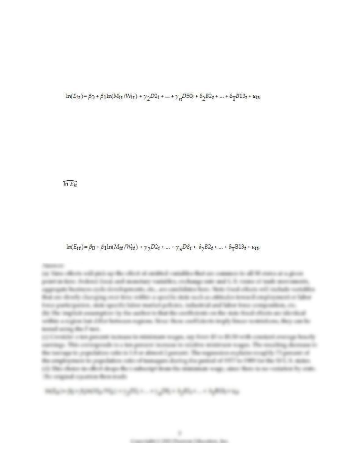
1) A study, published in 1993, used U.S. state panel data to investigate the relationship between
minimum wages and employment of teenagers. The sample period was 1977 to 1989 for all 50 states. The
author estimated a model of the following type:
where E is the employment to population ratio of teenagers, M is the nominal minimum wage, and W is
average hourly earnings in manufacturing. In addition, other explanatory variables, such as the adult
unemployment rate, the teenage population share, and the teenage enrollment rate in school, were
included.
(a) Name some of the factors that might be picked up by time and state fixed effects.
(b) The author decided to use eight regional dummy variables instead of the 49 state dummy variables.
What is the implicit assumption made by the author? Could you test for its validity? How?
(c) The results, using time and region fixed effects only, were as follows:
= –0.182 × ln(Mit /Wit ) + …; R2= 0.727
(0.036)
Interpret the result briefly.
(d) State minimum wages do not exceed federal minimum wages often. As a result, the author decided to
choose the federal minimum wage in his specification above. How does this change your interpretation?
How is the original equation
affected by this?

2) You want to find the determinants of suicide rates in the United States. To investigate the issue, you
collect state level data for ten years. Your first idea, suggested to you by one of your peers from Southern
California, is that the annual amount of sunshine must be important. Stacking the data and using no fixed
effects, you find no significant relationship between suicide rates and this variable. (This is good news for
the people of Seattle.) However, sorting the suicide rate data from highest to lowest, you notice that those
states with the lowest population density are dominating in the highest suicide rate category. You run
another regression, without fixed effect, and find a highly significant relationship between the two
variables. Even adding some economic variables, such as state per capita income or the state
unemployment rate, does not lower the t–statistic for the population density by much. Adding fixed
entity and time effects, however, results in an insignificant coefficient for population density.
(a) What do you think is the cause for this change in significance? Which fixed effect is primarily
responsible? Does this result imply that population density does not matter?
(b) Speculate as to what happens to the coefficients of the economic variables when the fixed effects are
included. Use this example to make clear what factors entity and time fixed effects pick up.
(c) What other factors might play a role?

9
3) Two authors published a study in 1992 of the effect of minimum wages on teenage employment using
a U.S. state panel. The paper used annual observations for the years 1977–1989 and included all 50 states
plus the District of Columbia. The estimated equation is of the following type
(Eit )= β0 + β1 (Mit /Wit ) + D2i + … + D51i + B2t + … + B13t + uit,
where E is the employment to population ratio of teenagers, M is the nominal minimum wage, and W is
average wage in the state. In addition, other explanatory variables, such as the prime–age male
unemployment rate, and the teenage population share were included.
(a) Briefly discuss the advantage of using panel data in this situation rather than pure cross sections or
time series.
(b) Estimating the model by OLS but including only time fixed effects results in the following output
it = 0 – 0.33 × (Mit /Wit ) + 0.35(SHYit) – 1.53 × uramit; R2 = 0.20
(0.08) (0.28) (0.13)
where SHY is the proportion of teenagers in the population, and uram is the prime–age male
unemployment rate. Coefficients for the time fixed effects are not reported. Numbers in parenthesis are
homoskedasticity–only standard errors.
Comment on the above results. Are the coefficients statistically significant? Since these are level
regressions, how would you calculate elasticities?
(c) Adding state fixed effects changed the above equation as follows:
it = 0 + 0.07 × (Mit /Wit ) – 0.19 × (SHYit) – 0.54 × uramit; 2 = 0.69
(0.10) (0.22) (0.11)
Compare the two results. Why would the inclusion of state fixed effects change the coefficients in this
way?
(d) The significance of each coefficient decreased, yet 2 increased. How is that possible? What does this
result tell you about testing the hypothesis that all of the state fixed effects can be restricted to have the
same coefficient? How would you test for such a hypothesis?

11
4) You learned in intermediate macroeconomics that certain macroeconomic growth models predict
conditional convergence or a catch up effect in per capita GDP between the countries of the world. That
is, countries which are further behind initially in per–capita GDP will grow faster than the leader. You
gather data from the Penn World Tables to test this theory.
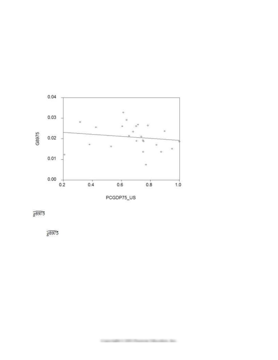
(a) By limiting your sample to 24 OECD countries, you hope to have a more homogeneous set of
countries in your sample, i.e., countries that are not too different with respect to their institutions. To
simplify matters, you decide to only test for unconditional convergence. In that case, the laggards catch
up even without taking into account differences in some of the driving variables. Your scatter plot and
regression for the time period 1975–1989 are as follows:
= 0.024 – 0.005 PCGDP75_US; R2= 0.025, SER = 0.006
(0.06) (0.008)
where is the average annual growth rate of per capita GDP from 1975–1989, and PCGDP75_US is
per capita GDP relative to the United States in 1975. Numbers in parenthesis are heteroskedasticity–
robust standard errors.
12
Interpret the results. Is there indication of unconditional convergence? What critical value did you use?
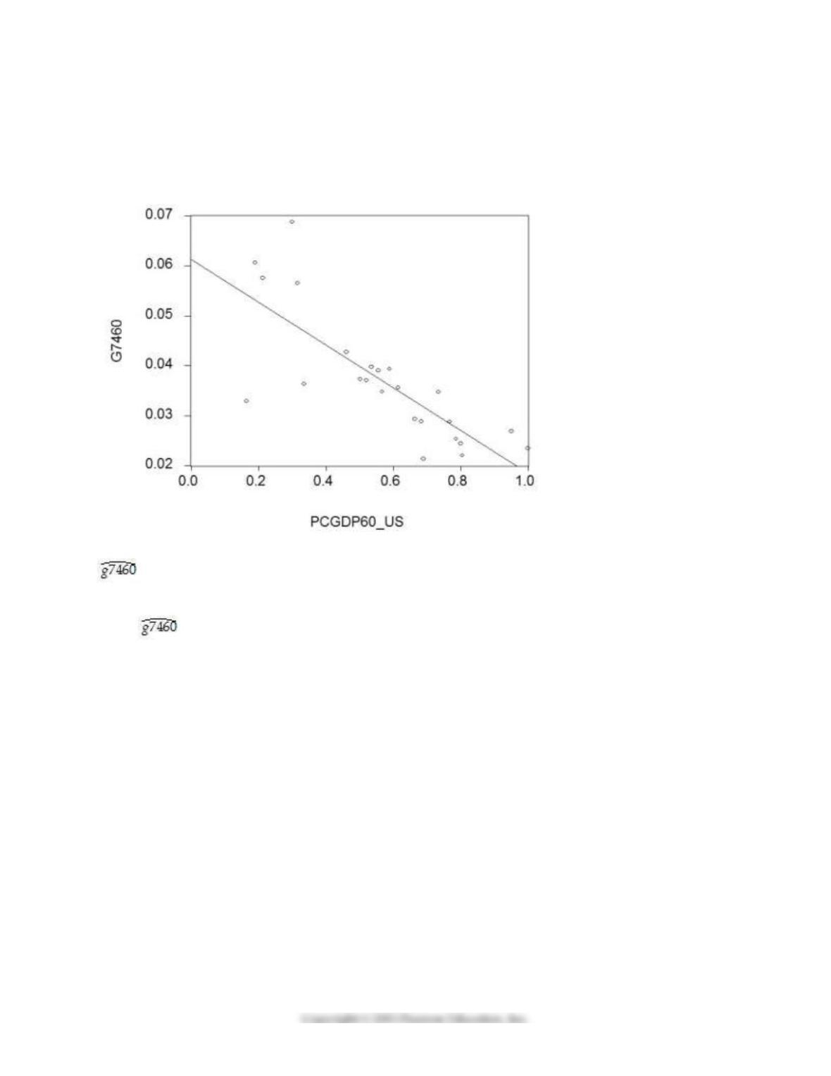
(b) Although you are quite discouraged by the result, you think that it might be due to the specific time
period used. During this period, there were two OPEC oil price shocks with varying degrees of exposure
for the OECD countries. You therefore repeat the exercise for the period 1960–1974, with the following
results:
= 0.061 – 0.043 PCGDP60_US; R2= 0.613, SER = 0.008
(0.004) (0.007)
where is the average annual growth rate of per capita GDP from 1960–1974, and PCGDP60_US is
per capita GDP relative to the United States in 1960.
Compare this regression to the previous one.
(c) You decide to run one more regression in differences. The dependent variable is now the change in the
growth rate of per capita GDP from 1960–1974 to 1975–1989 (diffg) and the regressor the difference in the
initial conditions (diffinit). This produces the following graph and regression:
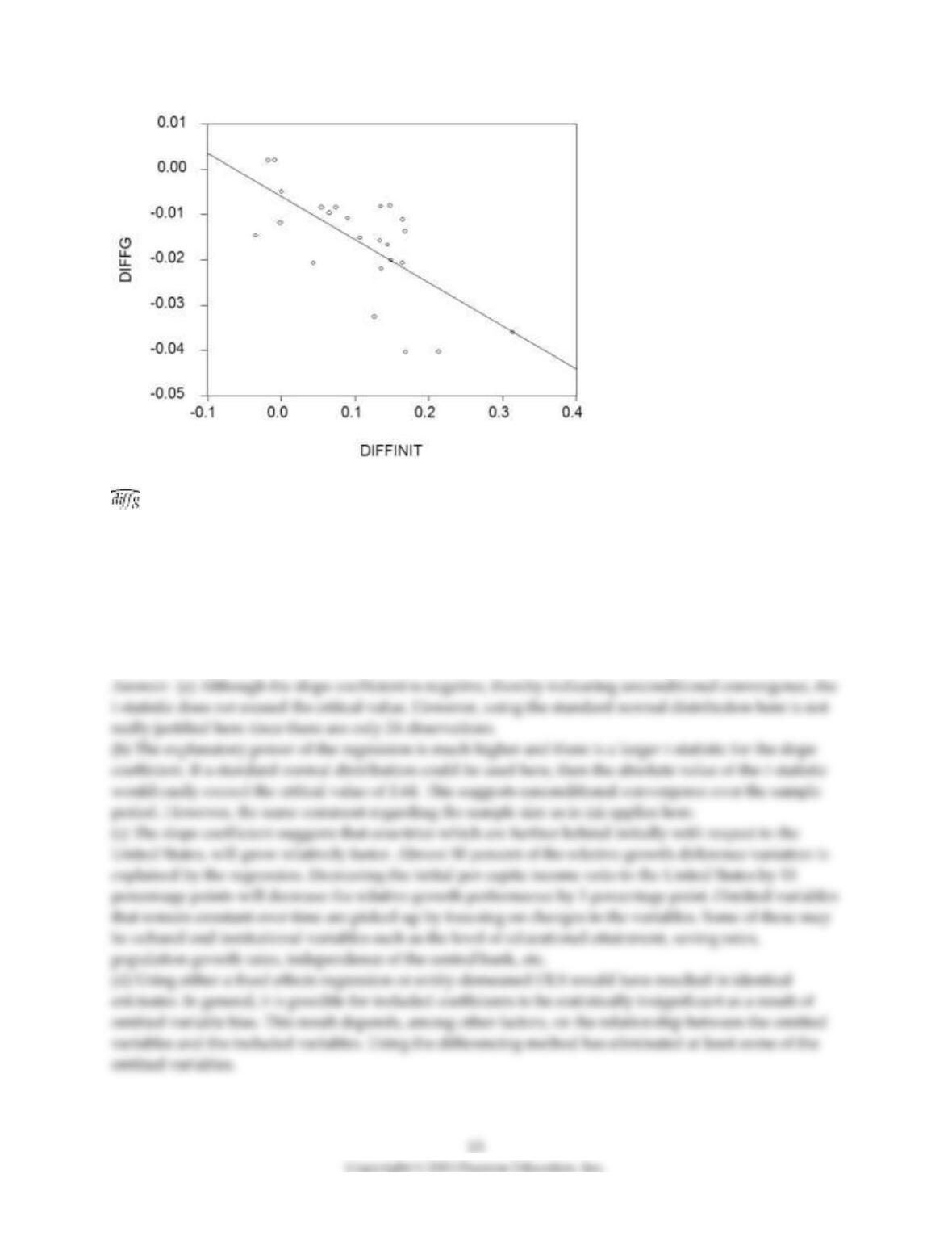
= –0.006 – 0.096 × diffinit; R2 = 0.468; SER = 0.009
(0.03) (0.021)
Interpret these results. Explain what has happened to unobservable omitted variables that are constant
over time. Suggest what some of these variables might be.
(d) Given that there are only two time periods, what other methods could you have employed to generate
the identical results? Why do you think that the slope coefficient in this regression is significant given the
results over the sub–periods?