imports, then a decline in government spending by $60 million will result in a total reduction in equilibrium income of:
a.
$171.43 million.
b.
$123.47 million.
c.
$151.63 million.
d.
$73.47 million.
e.
$71.43 million.
59. Suppose equilibrium income in an economy decreases by $600 as a result of a change in government spending. If the
multiplier is 3, what is the change in government spending?
a.
Government spending will decrease by $1,800.
b.
Government spending will decrease by $600.
c.
Government spending will decrease by $200.
d.
Government spending will increase by $400.
e.
Government spending will increase by $1,200.
MACR.BOYE.16.51 – ch. 10, 5
Changes in Equilibrium Income and Expenditures
60. Consider a closed economy described by AE (aggregate expenditures) = 800,000 + 0.75Y Assume that this economy
is initially in equilibrium. But now the government implements a program to improve highways that will cost $1 million.
This implies that equilibrium real GDP will:
a.
decrease by $1 million.
b.
decrease by $4 million.
c.
increase by $1 million.
d.
increase by $4 million.
e.
decrease by $800,000.
MACR.BOYE.16.52 – ch. 10, 6
United States – Reflective Thinking
Changes in Equilibrium Income and Expenditures
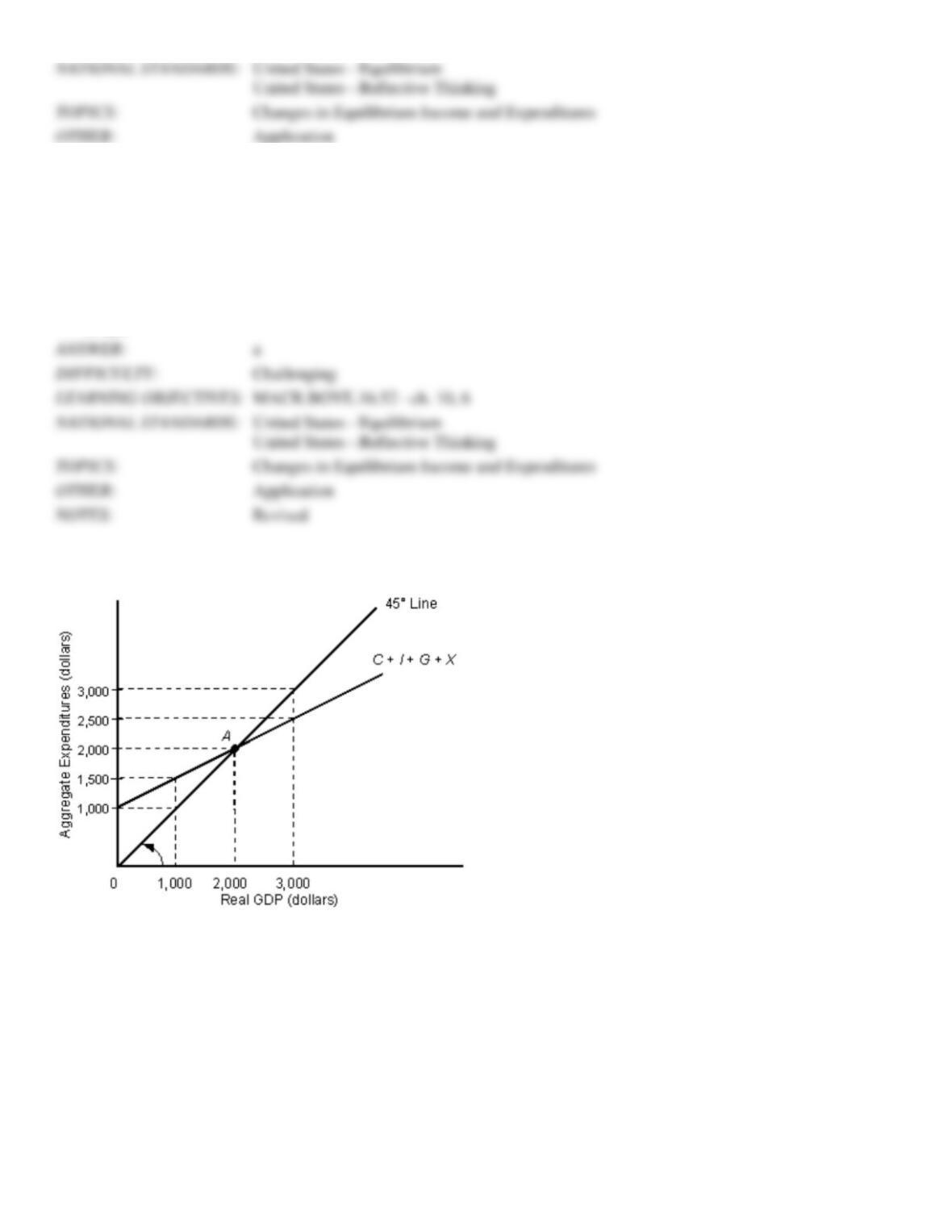
The figure given below represents the macroeconomic equilibrium in the aggregate income and aggregate expenditure
MACR.BOYE.16.51 – ch. 10, 5
Changes in Equilibrium Income and Expenditures
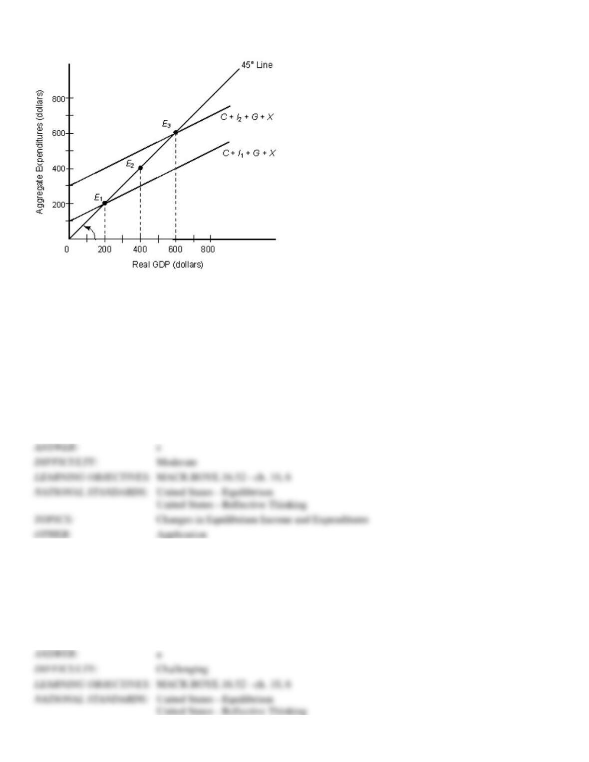
framework. Assume that MPI is equal to zero.
Figure 10.4
In the figure:
C: Consumption
I1 and I2: Investment
G: Government Spending
X: Net Exports
61. Refer to Figure 10.4. Compute the increase in investment spending from I1 to I2.
a.
$600
b.
$100
c.
$200
d.
$400
e.
$300
62. Refer to Figure 10.4. The spending multiplier is _____.
a.
2
b.
3
c.
6
d.
0.5
e.
1.2
MACR.BOYE.16.52 – ch. 10, 6
Moderate
MACR.BOYE.16.52 – ch. 10, 6
Changes in Equilibrium Income and Expenditures
Application
63. In Figure 10.4, calculate the marginal propensity to consume.
a.
0.67
b.
0.50
c.
0.25
d.
0.33
e.
4
b
Challenging
MACR.BOYE.16.52 – ch. 10, 6
United States – Reflective Thinking
Changes in Equilibrium Income and Expenditures
Application
64. Refer to Figure 10.4. Assume that the economy is initially at the equilibrium level E3. The economy can reach
equilibrium level E1 if aggregate expenditure:
a.
decreases by $200.
b.
increases by $200.
c.
decreases by $100.
d.
increases by $100.
e.
increases by $50.
Moderate
MACR.BOYE.16.52 – ch. 10, 6
United States – Reflective Thinking
Changes in Equilibrium Income and Expenditures
Application
Revised
65. Refer to Figure 10.4. If autonomous government expenditures increase by $250 billion, equilibrium real GDP will:
a.
rise by $250 billion.
b.
fall by 300 billion.
c.
rise by $500 billion.
d.
rise by $75 billion.
e.
rise by $100 billion.
Moderate
MACR.BOYE.16.52 – ch. 10, 6
United States – Reflective Thinking
Application
Changes in Equilibrium Income and Expenditures
Application
66. If the spending multiplier equals 5 and equilibrium income is $2 billion below potential GDP, then _____ to reach the
potential real GDP level.
a.
total spending needs to increase by $0.1 billion
b.
nominal GDP needs to increase by $1.2 billion
c.
total spending needs to decrease by $6 billion
d.
nominal GDP needs to decrease by $12 billion
e.
total spending needs to increase by $0.4 billion
67. Assume that a GDP gap can be closed by a $200 initial change in planned spending. The MPS is 0.3 and the MPI
equals 0.1. If the economy is currently in equilibrium with an income level of $600, potential GDP equals:
a.
$1,600.
b.
$1,100.
c.
$800.
d.
$600.
e.
$400.
Challenging
MACR.BOYE.16.52 – ch. 10, 6
Changes in Equilibrium Income and Expenditures
Application
68. Assume that potential GDP is $200 billion and the multiplier equals 5. The recessionary gap is $10 billion. What is the
actual level of equilibrium income?
a.
$200 billion
b.
$150 billion
c.
$100 billion
d.
$80 billion
e.
$50 billion
b
Challenging
MACR.BOYE.16.52 – ch. 10, 6
Changes in Equilibrium Income and Expenditures
Moderate
MACR.BOYE.16.52 – ch. 10, 6
United States – Reflective Thinking
Application
Revised
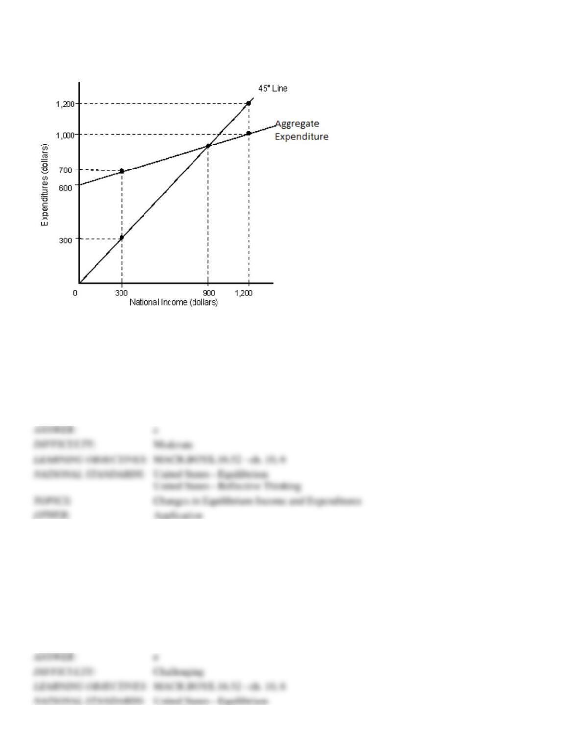
The figure given below depicts macroeconomic equilibrium in a closed economy. Assume that the spending multiplier in
this economy is 1.5.
Figure 10.5
69. Refer to Figure 10.5. If the target or potential level of real GDP is $1,200, then at an equilibrium real GDP level of
$900:
a.
the GDP gap is zero.
b.
there exists a recessionary gap that could be closed by a $200 decrease in planned aggregate expenditures.
c.
the GDP gap is $200.
d.
actual real GDP exceeds potential real GDP by $300.
e.
there exists a recessionary gap that could be closed by a $200 increase in autonomous investment spending.
70. Refer to Figure 10.5. Assume that there is a recessionary gap that can be closed by a $500 increase in planned
aggregate expenditures. If the economy is initially in equilibrium with a real GDP level of $900, then the target or
potential level of real GDP must be:
a.
$333.33.
b.
$400.
c.
$750.
d.
$1,400.
e.
$1,650.
Challenging
Moderate
MACR.BOYE.16.52 – ch. 10, 6
Changes in Equilibrium Income and Expenditures
Application
71. Refer to Figure 10.5. Suppose that the economy is characterized by an equilibrium real GDP level of $900 that
exceeds the potential real GDP level by $600. This so-called expansionary gap can be closed by:
a.
increasing planned aggregate expenditures by $400.
b.
lowering government purchases by $600.
c.
lowering autonomous consumption spending by $400.
d.
increasing planned aggregate expenditures by $900.
e.
lowering autonomous net exports by $600.
Challenging
MACR.BOYE.16.52 – ch. 10, 6
United States – Reflective Thinking
Changes in Equilibrium Income and Expenditures
Application
Revised
The table given below shows the real GDP, aggregate expenditures, saving, and imports of an economy.
Table 10.4
Real GDP
Aggregate
Expenditures
Saving
Imports
$0
$800
–$300
$50
$1,000
$1,600
−$200
$150
$2,000
$2,400
−$100
$250
$3,000
$3,200
$0
$350
$4,000
$4,000
$100
$450
$5,000
$4,800
$200
$550
$6,000
$5,600
$300
$650
72. Refer to Table 10.4. Suppose the economy is currently in equilibrium and has a potential GDP of $6,000. The current
GDP gap equals _____.
a.
$400
b.
$1,000
c.
$2,000
d.
$3,000
e.
$6,000
Moderate
MACR.BOYE.16.52 – ch. 10, 6
United States – Reflective Thinking
Application
73. Refer to Table 10.4. Given a potential GDP of $6,000, the recessionary gap equals _____.
United States – Reflective Thinking
Changes in Equilibrium Income and Expenditures
Application
a.
$200
b.
$400
c.
$1,000
d.
$2,000
e.
$5,000
74. Calculate the marginal propensity to save for the economy from the information given in Table 10.4.
a.
0.9
b.
0.8
c.
0.5
d.
0.2
e.
0.1
Moderate
MACR.BOYE.16.52 – ch. 10, 6
Changes in Equilibrium Income and Expenditures
Application
75. Calculate the spending multiplier from the information given in Table 10.4.
a.
5
b.
4
c.
2
d.
0.2
e.
0.1
Challenging
MACR.BOYE.16.51 – ch. 10, 5
United States – Reflective Thinking
Changes in Equilibrium Income and Expenditures
Application
76. Calculate the marginal propensity to consume for the economy from the information given in Table 10.4.
a.
0.9
b.
0.8
c.
0.5
d.
0.2
b
Challenging
MACR.BOYE.16.52 – ch. 10, 6
United States – Reflective Thinking
Changes in Equilibrium Income and Expenditures
Application
e.
0.1
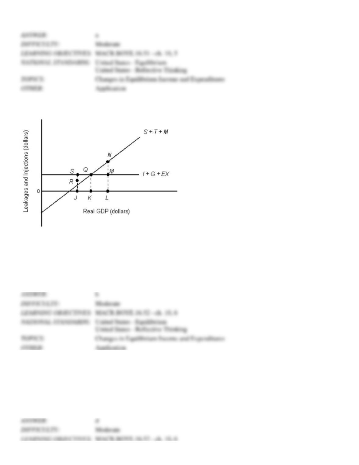
The figure given below represents the leakages and injections in an economy.
Figure 10.6
77. In Figure 10.6, the economy is in equilibrium at point _____.
a.
S
b.
Q
c.
N
d.
R
e.
M
b
Moderate
MACR.BOYE.16.52 – ch. 10, 6
Application
78. In Figure 10.6, if 0L is the potential level of real GDP, then KL represents:
a.
excess GDP.
b.
real GDP.
c.
the multiplier effect.
d.
the GDP gap.
e.
the recessionary gap.
d
MACR.BOYE.16.52 – ch. 10, 6
Moderate
MACR.BOYE.16.51 – ch. 10, 5
Changes in Equilibrium Income and Expenditures
Application
79. Refer to Figure 10.6. If 0L represents potential GDP, then the GDP gap can be closed by increasing autonomous
expenditures by an amount equal to the line segment _____.
a.
NM
b.
NL
c.
ML
d.
OK
e.
QK
MACR.BOYE.16.52 – ch. 10, 6
Changes in Equilibrium Income and Expenditures
Application
Revised
The figure given below shows the macroeconomic equilibrium of a country.
Figure 10.7
In the figure,
C: Consumption
I: Investment
G: Government expenditure
X: Net Exports
80. Refer to Figure 10.7. What is the size of the GDP gap if potential GDP equals $3,000?
a.
$500
b.
$1,000
c.
$2,000
d.
$2,500
e.
$3,000
Application
81. Given a potential GDP level of $3,000, the recessionary gap in Figure 10.7 equals _____.
a.
$3,000
b.
$2,500
c.
$1,500
d.
$500
e.
$100
d
Moderate
MACR.BOYE.16.52 – ch. 10, 6
Changes in Equilibrium Income and Expenditures
Application
82. In Figure 10.7, the spending multiplier equals _____.
a.
2
b.
4
c.
5
d.
10
e.
20
Challenging
MACR.BOYE.16.52 – ch. 10, 6
United States – Reflective Thinking
Changes in Equilibrium Income and Expenditures
Application
83. If a country’s imports are very important in determining the volume of exports from its trading partners, then:
a.
the simple spending multiplier understates the true value of the multiplier.
b.
the spending multiplier will be equal to 1/marginal propensity to import.
c.
the simple spending multiplier is an accurate measure of the multiplier effect.
d.
the simple spending multiplier will be equal to 1/MPC
e.
the spending multiplier will be equal to 1/marginal propensity to save.
Moderate
MACR.BOYE.16.53 – ch. 10, 7
b
Moderate
MACR.BOYE.16.52 – ch. 10, 6
United States – Reflective Thinking
Changes in Equilibrium Income and Expenditures
Application
84. The spending multiplier equals 1/marginal propensity to save if an economy:
a.
has a trade surplus.
b.
is open to international trade.
c.
does not trade with any other country.
d.
has a higher level of saving than consumption.
e.
reduces its investment expenditures to zero.
MACR.BOYE.16.53 – ch. 10, 7
United States – Equilibrium
United States – Reflective Thinking
Changes in Equilibrium Income and Expenditures
85. Foreign repercussions of changes in domestic spending may cause:
a.
the GDP gap to be larger than the recessionary gap.
b.
the equilibrium income to increase by an amount equal to the change in net exports.
c.
the actual spending multiplier to be larger than the reciprocal of the marginal propensity to save plus the
marginal propensity to import.
d.
equilibrium income to rise by a smaller amount than evidenced by the multiplier effect of autonomous
spending increase.
e.
the real GDP to be larger than potential GDP.
MACR.BOYE.16.53 – ch. 10, 7
United States – Analytic – BB-Legal
United States – Equilibrium
Changes in Equilibrium Income and Expenditures
86. Suppose only 7 percent of Turkey’s products go to the United States. Hence, an increase in U.S. imports from Turkey:
a.
would have no significant effect on Turkey’s domestic income.
b.
would significantly increase Turkey’s domestic income.
c.
would significantly decrease Turkey’s domestic income.
d.
would significantly increase U.S. domestic income.
e.
would significantly decrease U.S. domestic income.
United States – Reflective Thinking
Changes in Equilibrium Income and Expenditures
87. If 81 percent of Canada’s exports go to the United States, a recession in the United States would probably:
a.
lead to an economic boom in Canada.
b.
have no impact on Canada’s economy.
c.
increase imports from Canada.
d.
decrease Canada’s domestic real GDP.
e.
increase the per capita income in Canada.
d
Moderate
MACR.BOYE.16.53 – ch. 10, 7
United States – Equilibrium
Equilibrium Income and Expenditures
Application
Revised
88. Assume that the multiplier effect for Mexico is 0.85 for an increase in spending by the U.S. government by $1.
Therefore, a $20 billion decrease in spending by the U.S. government results in:
a.
a $23.5 billion increase in Mexican real GDP.
b.
a $133.3 billion decrease in Mexican real GDP.
c.
a $3 billion decrease in Mexican real GDP.
d.
a $17 billion decrease in Mexican real GDP.
e.
a $23.5 billion decrease in Mexican real GDP.
d
Moderate
MACR.BOYE.16.53 – ch. 10, 7
Changes in Equilibrium Income and Expenditures
Application
Revised
89. Suppose the marginal propensity to consume is 0.63, the marginal propensity to import equals 0.08, and personal
income taxes amount to 9 percent of GDP. The spending multiplier for this economy is equal to _____.
a.
0.54
b.
0.80
c.
1.25
d.
1.41
e.
1.85
Challenging
United States – Equilibrium
Application
90. The Keynesian aggregate expenditures model assumes that:
a.
production does not adjust to changes in aggregate expenditures.
b.
aggregate supply is autonomous.
c.
prices do not decrease when aggregate demand decreases.
d.
aggregate supply determines the equilibrium level of real GDP.
e.
prices are positively related to aggregate demand.
MACR.BOYE.16.54 – ch. 10, 8
United States – Equilibrium
Aggregate Expenditures and Aggregate Demand
91. A rise in the price level that reduces the real wealth of people who hold financial assets is an illustration of the:
a.
interest rate effect.
b.
monetary theory.
c.
supply-side theory.
d.
wealth effect.
e.
trade effect
MACR.BOYE.16.54 – ch. 10, 8
United States – Equilibrium
Aggregate Expenditures and Aggregate Demand
92. The interest rate effect states that an increase in the price level will cause:
a.
a decline in the interest rate.
b.
a decrease in investment and aggregate expenditures.
c.
an increase in the equilibrium level of income.
d.
a decrease in the supply of financial assets.
e.
an increase in real wealth.
MACR.BOYE.16.54 – ch. 10, 8
Aggregate Expenditures and Aggregate Demand
United States – Reflective Thinking
Changes in Equilibrium Income and Expenditures