5) A researcher investigating the determinants of crime in the United Kingdom has data for 42 police
regions over 22 years. She estimates by OLS the following regression
ln(cmrt)it = αi + φt + β1unrtmit + β2proythit + β3 ln(pp)it + uit; i = 1,…, t = 1,…, 22
where cmrt is the crime rate per head of population, unrtm is the unemployment rate of males, proyth is
the proportion of youths, pp is the probability of punishment measured as (number of
convictions)/(number of crimes reported). α and φ are area and year fixed effects, where αi equals one for
area i and is zero otherwise for all i, and φt is one in year t and zero for all other years for t = 2, …, 22. φ1
is not included.
(a) What is the purpose of excluding φ1? What are the terms α and φ likely to pick up? Discuss the
advantages of using panel data for this type of investigation.
(b) Estimation by OLS using heteroskedasticity and autocorrelation–consistent standard errors results in
the following output, where the coefficients of the fixed effects are not reported:
= 0.063 × unrtmit + 3.739 × proythit – 0.588 × ln(pp)it ; R2 = 0.904
(0.109) (0.179) (0.024)
Comment on the results. In particular, what is the effect of a ten percent increase in the probability of
punishment?
(c) To test for the relevance of the area fixed effects, your restrict the regression by dropping all entity
fixed effects and add single constant is added. The relevant F–statistic is 135.28. What are the degrees of
freedom? What is the critical value from your F table?
(d) Although the test rejects the hypothesis of eliminating the fixed effects from the regression, you want
to analyze what happens to the coefficients and their standard errors when the equation is re–estimated
without fixed effects. In the resulting regression, and do not change by much, although their
standard errors roughly double. However, is now 1.340 with a standard error of 0.234. Why do you
think that is?

6) You want to investigate the relationship between cumulative GPA scores at graduation and incoming
SAT scores of students. For this purpose, you have collected data from a balanced panel of 120
undergraduate colleges and universities in the United States over a ten year period. Discuss some of the
entity fixed effects which you potentially capture by allowing for a binary variable for each of the
colleges.

7) You want to study the relationship between weight and height of young children (4th grade to 7th
grade). You collect data for more than 400 students and track the progress of these students over the
following four years, where you end up with a balanced panel of 400 students (you discard the
observations for the students who moved away). Discuss some of the entity fixed effects which you
potentially capture by allowing for a binary variable for each of the students. Do you expect significant
time fixed effects if you allowed for them?
8) You first encountered growth regression in your intermediate macroeconomics course (“beta–
convergence regressions”), that is, conditionally on some initial condition in per capita income, different
authors tried to find the determinants of growth. Since growth is a long–run phenomenon, various
studies collected data for a panel of numerous countries using 10–year averages, over a time period
stretching from 1960 to 2005. For example, a balanced panel might consist of 50 or so odd countries for
the time periods 1960–1970, 1971–1980, …, 2000–2005. Instead of using two–way fixed effects (entity fixed
effects and time fixed) authors often only employed time fixed effects. Why do you think that is? What
sort of information would be lost if these authors employed entity fixed effects as well?
1) Your textbook suggests an “entity–demeaned” procedure to avoid having to specify a potentially large
number of binary variables. While it is somewhat tedious to specify a binary variable for each entity, this
can still be handled relatively easily in the case of the 48 contiguous states. Give a few examples where it
might be close to impossible to implement specifying such large number of entity binary variables. The
idea of the “entity–demeaned” procedure was introduced as a computationally convenient and
simplifying procedure. Since there are also time fixed effects, why is there no discussion of using a “time–
demeaned” procedure? Using the following equation
Yit = β0 + β1Xit + β3St + uit,
Show how β1 can be estimated by the OLS regression using “time–demeaned” variables.
2) Consider the case of time fixed effects only, i.e.,
Yit = β0 + β1Xit + β3St + uit,
First replace β0 + β3St with φt. Next show the relationship between the φt and δt in the following
equation
Yit = β0 + β1Xit + δ2B2t + … + δTBTt + uit,
where each of the binary variables B2, …, BT indicates a different time period. Explain in words why the
two equations are the same. Finally show why there is perfect multicollinearity if you add another binary
variable B1. What is the intuition behind the fact that the OLS estimator does not exist in this case? Would
that also be the case if you dropped the intercept?

3) Consider the following panel data regression with a single explanatory variable
Yit = β0 + β1Xit + uit.
In each of the examples below, you will be adding entity and time fixed effects. Indicate the total number
of coefficients that need to be estimated.
(a) The effect of beer taxes on the fatality rate, annual data, 1982–1988, nine U.S. regions (New England,
Pacific, Mid–Atlantic, East North Central, etc.).
(b) The effect of the minimum wage on teenage employment, annual data, 1963–2000, five Canadian
Regions (Atlantic Provinces, Quebec, Ontario, Prairies, British Columbia).
(c) The effect of savings rates on per capita income, data for three decades (1960–1969, 1970–1979, 1980–
1989; one observation per decade), 104 countries of the world.
(d) The effect of pitching quality in baseball (as measured by the Team ERA) on the winning percentage,
annual data, 1998–1999 season, 1999–2000 season, 30 teams.
4) Your textbook modifies the four assumptions for the multiple regression model by adding a new
assumption. This represents an extension of the cross–sectional data case, where errors are uncorrelated
across entities. The new assumption requires the errors to be uncorrelated across time, conditional on the
regressors as well (cov(uit, uis Xit, Xis) = 0 for t ≠ s.).
(a) Discuss why there might be correlation over time in the errors when you use U.S. state panel data.
Does this mean that you should not use OLS as an estimator?
(b) Now consider pairs of adjacent states such as Indiana and Michigan, Texas and Arkansas, New York
and Connecticut, etc. Is it likely that the fifth assumption will hold here, even though the
“contemporaneous” errors are correlated? If not, can you still use OLS for estimation?
5) In Sports Economics, production functions are often estimated by relating the winning percentage of
teams (Y) to inputs indicating performance in certain aspects of the game. However, this omits the quality
of management. Assume that you could measure the quality of pitching and hitting by a single index L,
and that managerial ability is represented by M, which is assumed to be constant over time. The
production function would then be specified as follows:
Yit = β0 +β1 Lit + β2Mi + uit
where i is an index for the baseball team, and t indexes time and all variables are in logs.
(a) Assume that managerial ability is unobservable but is positively related, in a linear way, to L. Explain
why the OLS estimator 1 is inconsistent in the case of a single cross–section, i.e., if you attempt to
estimate the above regression for a single year. Do you expect this coefficient to over– or under–estimate
β1?
(b) If you had data for two years, indicate the transformation, which allows you to obtain a consistent
estimator for β1.

6) A study attempts to investigate the role of the various determinants of regional Canadian
unemployment rates in order to get a better picture of Canadian aggregate unemployment rate behavior.
The annual data (1967–1991) is for five regions (Atlantic region, Quebec, Ontario, Prairies, and British
Columbia), and four age–gender groups (female and male, adult and young). Focusing on young females,
the authors find significant effects for the following variables: the regional relative minimum wage rate
(minimum wages divided by average hourly earnings), the regional share of youth in the labor force, the
regional share of adult females in the labor force, United States activity shocks (deviations of United
States GDP from trend), an indicator of the degree of monetary tightness in Canada, regional union
density, and a regional index of unemployment insurance generosity. Explain why the authors only used
region fixed effects. How would their specification have to change if they also employed time fixed
effects?
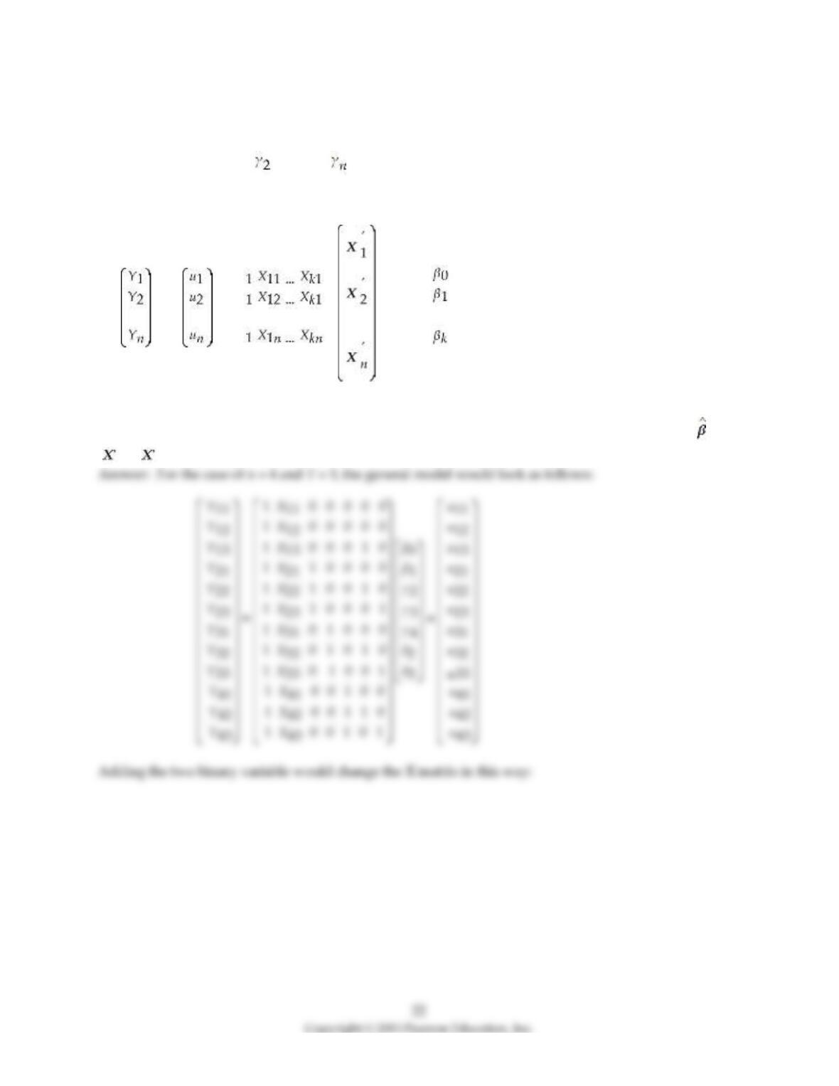
7) (Requires Matrix Algebra) Consider the time and entity fixed effect model with a single explanatory
variable
Yit = β0 + β1Xit + D2i + ... + Dni + δ2B2t + … + δTBTt + uit,
For the case of n = 4 and T = 3, write this model in the form Y = Xβ + U, where, in general,
Y = , U = , X = = , and β =
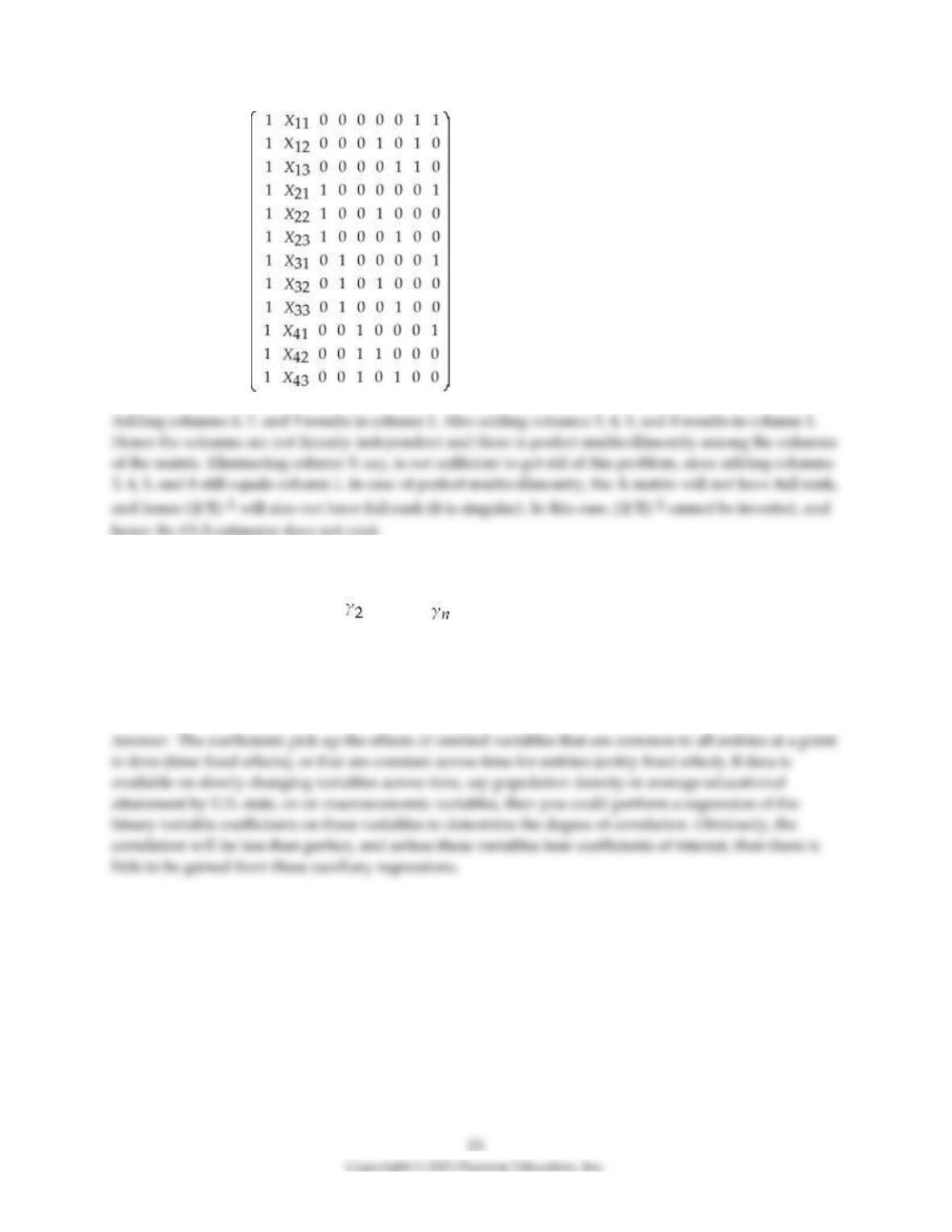
How would the X matrix change if you added two binary variables, D1 and B1? Demonstrate that in this
case the columns of the X matrix are not independent. Finally show that elimination of one of the two
variables is not sufficient to get rid of the multicollinearity problem. In terms of the OLS estimator, =
(X)–1Y, why does perfect multicollinearity create a problem?
X =
8) Consider the time and entity fixed effect model with a single explanatory variable
Yit = β0 + β1Xit + D2i + ... + Dni + δ2B2t + … + δTBTt + uit,
Assume that you had estimated the above equation by OLS. Typically the coefficients for the entity and
time binary variables are not reported. Can you think of situations where the pattern of these coefficients
might be of interest? What could you do, for example, if you had a strong theoretical justification for
believing that a few macroeconomic variables had an effect on Yit?

9) “Empirical studies of economic growth are flawed because many of the truly important underlying
determinants, such as culture and institutions, are very hard to measure.” Discuss this statement paying
particular attention to simple cross–section data and panel data models. Use equations whenever possible
to underscore your argument.
10) Give at least three examples from macroeconomics and five from microeconomics that involve
specified equations in a panel data analysis framework. Indicate in each case what the role of the entity
and time fixed effects in terms of omitted variables might be.

11) Your textbook specifies a simple regression problem for two time periods for the years 1982 and 1988
as follows:
FatalityRatei,1982 = β0 + β1BeerTaxi,1982 + ui,1982
FatalityRatei,1988 = β0 + β1BeerTaxi,1988 + ui,1988
After subtracting the first equation from the second equation, the authors estimate the model and find a
negative intercept.
a. Show how you would have to modify the two equations to allow for the presence of an intercept in the
differenced model.
b. What would the relative magnitude of the modified model have to be for you to find a negative
intercept?
12) Your textbook reports the following result from an two–way fixed effects (entity and time fixed
effects) regression model:
= –0.66 BeerTax + StateFixedEffects + TimeFixedEffects
(0.36)
Where the number in parenthesis is the heteroskedasticity– and autocorrelation–consistent (HAC)
standard error.
a. Calculate the t–statistic. Can you reject the null hypothesis that the slope coefficient is zero in the
population, using a two–sided test and a 5% significance level?
b. Given that economic theory suggests that the population slope is negative under the alternative
hypothesis, is it possible to use a one–sided test here? In that case, does your conclusion change?
c. Using only heteroskedasticity–robust standard errors, but not HAC standard errors, the value in
parenthesis becomes 0.25. Repeat the calculations in (a) and report your decision based on a two–sided
test.
d. Since the coefficient becomes more statistically significant in (d), should this influence your choice of
standard errors? Why or why not?