Ch.4 DescribingtheRelationbetweenTwoVariables
4.1 ScatterDiagramsandCorrelation
1 Drawandinterpretscatterdiagrams.
SHORTANSWER.Writethewordorphrasethatbestcompleteseachstatementoranswersthequestion.
Constructascatterdiagramforthedata.
1) Thedatabelowarethefinalexamscoresof10randomlyselectedhistorystudentsandthenumberofhours
theystudiedfortheexam.
Hours,x
Scores,y
3
65
5
80
2
60
8
88
2
66
4
78
4
85
5
90
6
90
3
71
x
y
x
y
2) Thedatabelowarethetemperaturesonrandomlychosendaysduringasummerclassandthenumberof
absencesonthosedays.
Temperature,x
Numberofabsences,y
72
3
85
7
91
10
90
10
88
8
98
15
75
4
100
15
80
5
x
y
x
y
Page83
3) Thedatabelowaretheagesandsystolicbloodpressures(measuredinmillimetersofmercury)of9randomly
selectedadults.
Age,x
Pressure,y
38
116
41
120
45
123
48
131
51
142
53
145
57
148
61
150
65
152
x
y
x
y
4) Thedatabelowarethenumberofabsencesandthefinalgradesof9randomlyselectedstudentsfroma
literatureclass.
Numberofabsences,x
Finalgrade,y
0
98
3
86
6
80
4
82
9
71
2
92
15
55
8
76
5
82
x
y
x
y
Page84
5) Amanagerwishestodeterminetherelationshipbetweenthenumberofmiles(inhundredsofmiles)the
managerʹssalesrepresentativestravelpermonthandtheamountofsales(inthousandsofdollars)permonth.
Milestraveled,x
Sales,y
2
31
3
33
10
78
7
62
8
65
15
61
3
48
1
55
11
120
x
y
x
y
6) Inorderforemployeesofacompanytoworkinaforeignoffice,theymusttakeatestinthelanguageofthe
countrywheretheyplantowork.Thedatabelowshowtherelationshipbetweenthenumberofyearsthat
employeeshavestudiedaparticularlanguageandthegradestheyreceivedontheproficiencyexam.
Numberofyears,x
Gradesontest,y
3
61
4
68
4
75
5
82
3
73
6
90
2
58
7
93
3
72
x
y
x
y
Page85
7) InanareaoftheGreatPlains,recordswerekeptontherelationshipbetweentherainfall(ininches)andthe
yieldofwheat(bushelsperacre).
Rainfall(ininches),x
Yield(bushelsperacre),y
10.5
50.5
8.8
46.2
13.4
58.8
12.5
59.0
18.8
82.4
10.3
49.2
7.0
31.9
15.6
76.0
16.0
78.8
x
y
x
y
8) Fivebrandsofcigarettesweretestedfortheamountsoftarandnicotinetheycontained.Allmeasurementsare
inmilligramspercigarette.
Cigarette Tar Nicotine
BrandA 16 1.2
BrandB 13 1.1
BrandC 16 1.3
BrandD 18 1.4
BrandE 6 0.6
x
y
x
y
9) Thescoresofninemembersofalocalcommunitycollegewomenʹsgolfteamintworoundsoftournamentplay
arelistedbelow.
Player 123456789
Round1859087789285799386
Round2908785848678779182
x
y
x
y
Page86
MULTIPLECHOICE.Choosetheonealternativethatbestcompletesthestatementoranswersthequestion.
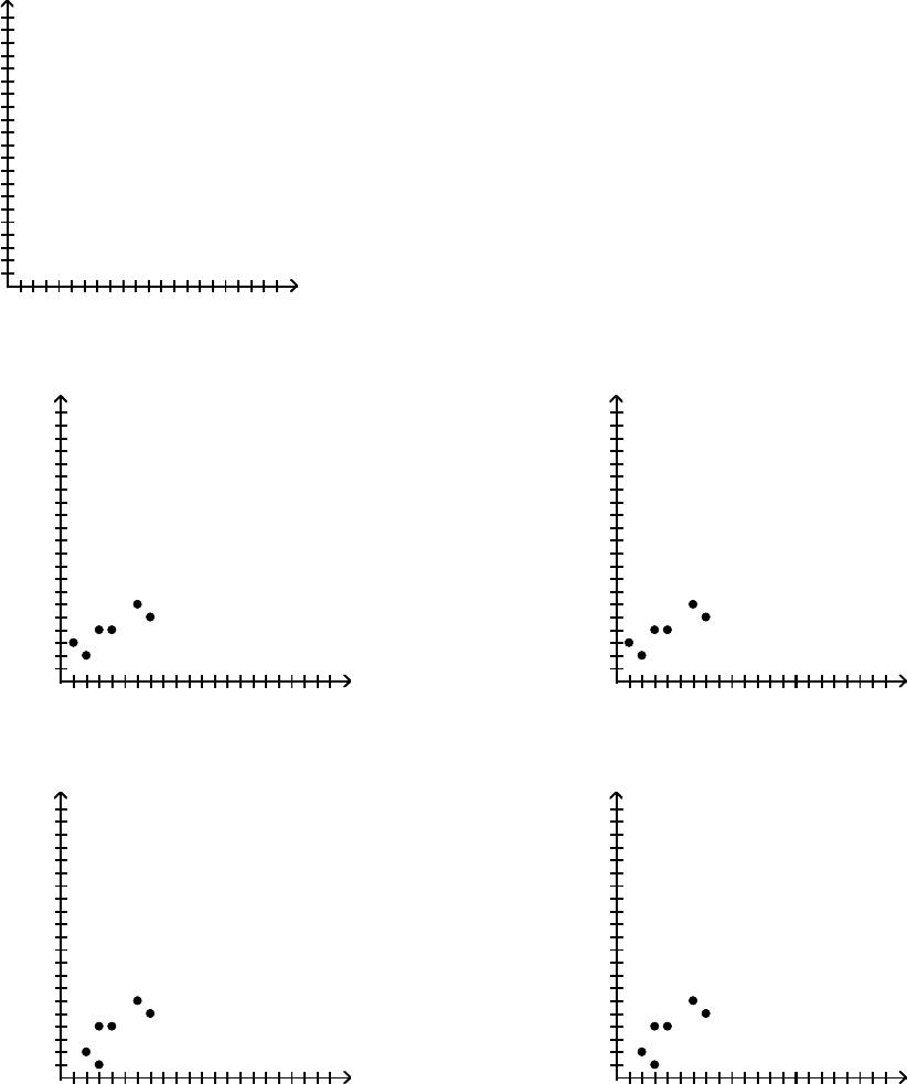
Makeascatterdiagramforthedata.Usethescatterdiagramtodescribehow,ifatall,thevariablesarerelated.
10) x164372
y 364452
x
2 4 6 8 10 12 14 16 18 20
y
20
18
16
14
12
10
8
6
4
2
x
2 4 6 8 10 12 14 16 18 20
y
20
18
16
14
12
10
8
6
4
2
A) Thevariablesappeartobe
positively,linearlyrelated.
x
2 4 6 8 10 12 14 16 18 20
y
20
18
16
14
12
10
8
6
4
2
x
2 4 6 8 10 12 14 16 18 20
y
20
18
16
14
12
10
8
6
4
2
B) Thevariablesdonotappeartobe
linearlyrelated.
x
2 4 6 8 10 12 14 16 18 20
y
20
18
16
14
12
10
8
6
4
2
x
2 4 6 8 10 12 14 16 18 20
y
20
18
16
14
12
10
8
6
4
2
C) Thevariablesappeartobe
negatively,linearlyrelated.
x
2 4 6 8 10 12 14 16 18 20
y
20
18
16
14
12
10
8
6
4
2
x
2 4 6 8 10 12 14 16 18 20
y
20
18
16
14
12
10
8
6
4
2
D) Thevariablesdonotappeartobe
linearlyrelated.
x
2 4 6 8 10 12 14 16 18 20
y
20
18
16
14
12
10
8
6
4
2
x
2 4 6 8 10 12 14 16 18 20
y
20
18
16
14
12
10
8
6
4
2
Page87
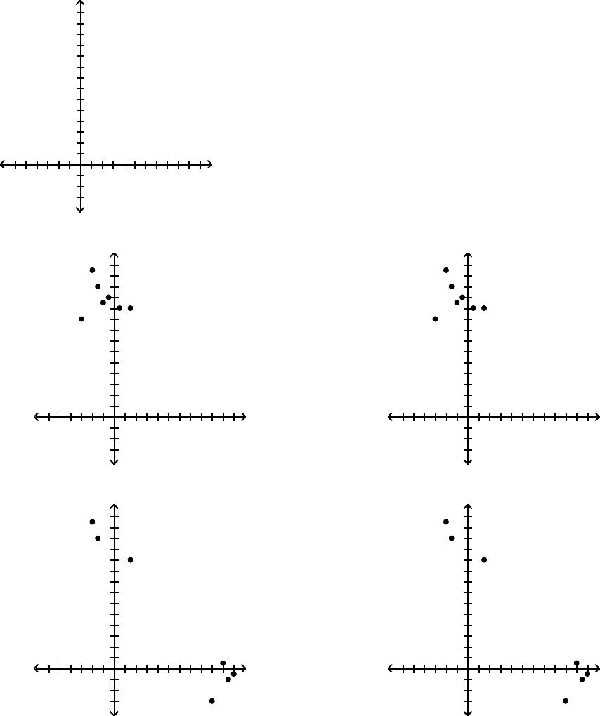
11) x1–1–6–2–33–4
y2022 18 21 24 20 27
x
–12–8–4 4 8 121620
y
28
24
20
16
12
8
4
-4
x
–12–8–4 4 8 121620
y
28
24
20
16
12
8
4
-4
A) Thevariablesdonotappeartobe
linearlyrelated.
x
–12–8–4 4 8 121620
y
28
24
20
16
12
8
4
-4
x
–12–8–4 4 8 121620
y
28
24
20
16
12
8
4
-4
B) Thevariablesappeartobe
negatively,linearlyrelated.
x
–12–8–4 4 8 121620
y
28
24
20
16
12
8
4
-4
x
–12–8–4 4 8 121620
y
28
24
20
16
12
8
4
-4
C) Thevariablesdonotappeartobe
linearlyrelated.
x
–12–8–4 4 8 121620
y
28
24
20
16
12
8
4
-4
x
–12–8–4 4 8 121620
y
28
24
20
16
12
8
4
-4
D) Thevariablesappeartobe
positively,linearlyrelated.
x
–12–8–4 4 8 121620
y
28
24
20
16
12
8
4
-4
x
–12–8–4 4 8 121620
y
28
24
20
16
12
8
4
-4
Page88
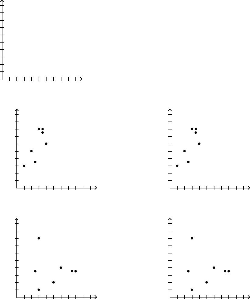
12)
Subject A B C D E F G
xTimewatchingTV 8427756
yTimeonInternet 12 10 615 16 716
x
2 4 6 8 10 12 14 16 18 20
y
20
18
16
14
12
10
8
6
4
2
x
2 4 6 8 10 12 14 16 18 20
y
20
18
16
14
12
10
8
6
4
2
A) Thevariablesappeartobe
positively,linearlyrelated.
x
2 4 6 8 10 12 14 16 18 20
y
20
18
16
14
12
10
8
6
4
2
x
2 4 6 8 10 12 14 16 18 20
y
20
18
16
14
12
10
8
6
4
2
B) Thevariablesdonotappeartobe
linearlyrelated.
x
2 4 6 8 101214161820
y
20
18
16
14
12
10
8
6
4
2
x
2 4 6 8 101214161820
y
20
18
16
14
12
10
8
6
4
2
C) Thevariablesappeartobe
negatively,linearlyrelated.
x
2 4 6 8 10 12 14 16 18 20
y
20
18
16
14
12
10
8
6
4
2
x
2 4 6 8 10 12 14 16 18 20
y
20
18
16
14
12
10
8
6
4
2
D) Thevariablesdonotappeartobe
linearlyrelated.
x
2 4 6 8 101214161820
y
20
18
16
14
12
10
8
6
4
2
x
2 4 6 8 101214161820
y
20
18
16
14
12
10
8
6
4
2
SHORTANSWER.Writethewordorphrasethatbestcompleteseachstatementoranswersthequestion.
Provideanappropriateresponse.
13) Anagriculturalbusinesswantstodetermineiftherainfallininchescanbeusedtopredicttheyieldperacreon
awheatfarm.Identifythepredictorvariableandtheresponsevariable.
14) Acollegecounselorwantstodetermineifthenumberofhoursspentstudyingforatestcanbeusedtopredict
thegradesonatest.Identifythepredictorvariableandtheresponsevariable.
Page89
MULTIPLECHOICE.Choosetheonealternativethatbestcompletesthestatementoranswersthequestion.
15) Thevariableisthevariablewhosevaluecanbeexplainedbythe variable.
A) response;predictor B) response;lurking
C) lurking;response D) predictorResponse
2 Describethepropertiesofthelinearcorrelationcoefficient.
MULTIPLECHOICE.Choosetheonealternativethatbestcompletesthestatementoranswersthequestion.
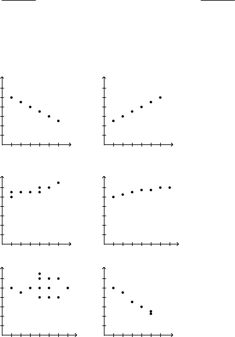
Usethescatterdiagramsshown,labeledathroughftosolvetheproblem.
1) Inwhichscatterdiagramisr=0.01?
a
x
123456
y
12
10
8
6
4
2
x
123456
y
12
10
8
6
4
2
b
x
123456
y
12
10
8
6
4
2
x
123456
y
12
10
8
6
4
2
c
x
123456
y
12
10
8
6
4
2
x
123456
y
12
10
8
6
4
2
d
x
1234567
y
12
10
8
6
4
2
x
1234567
y
12
10
8
6
4
2
e
x
1234567
y
12
10
8
6
4
2
x
1234567
y
12
10
8
6
4
2
f
x
123456
y
12
10
8
6
4
2
x
123456
y
12
10
8
6
4
2
A) e B) c C) f D) d
Page90
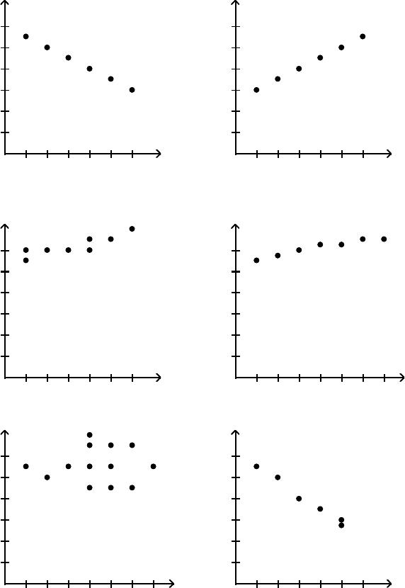
2) Inwhichscatterdiagramisr=1?
a
x
123456
y
12
10
8
6
4
2
x
123456
y
12
10
8
6
4
2
b
x
123456
y
12
10
8
6
4
2
x
123456
y
12
10
8
6
4
2
c
x
123456
y
12
10
8
6
4
2
x
123456
y
12
10
8
6
4
2
d
x
1234567
y
12
10
8
6
4
2
x
1234567
y
12
10
8
6
4
2
e
x
1234567
y
12
10
8
6
4
2
x
1234567
y
12
10
8
6
4
2
f
x
123456
y
12
10
8
6
4
2
x
123456
y
12
10
8
6
4
2
A)
b
B) a C) f D) d
Page91
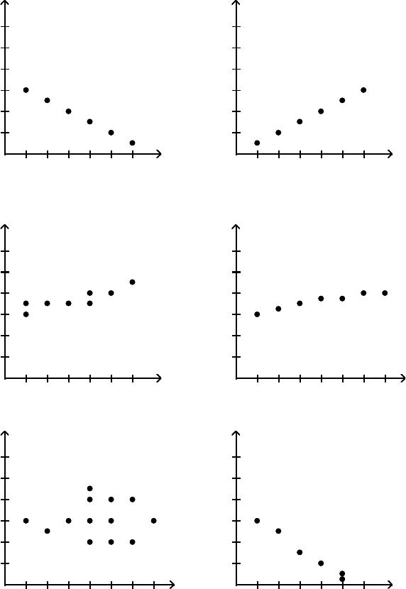
3) Inwhichscatterdiagramisr=–1?
a
x
123456
y
12
10
8
6
4
2
x
123456
y
12
10
8
6
4
2
b
x
123456
y
12
10
8
6
4
2
x
123456
y
12
10
8
6
4
2
c
x
123456
y
12
10
8
6
4
2
x
123456
y
12
10
8
6
4
2
d
x
1234567
y
12
10
8
6
4
2
x
1234567
y
12
10
8
6
4
2
e
x
1234567
y
12
10
8
6
4
2
x
1234567
y
12
10
8
6
4
2
f
x
123456
y
12
10
8
6
4
2
x
123456
y
12
10
8
6
4
2
A) a B)
b
C) f D) d
Page92
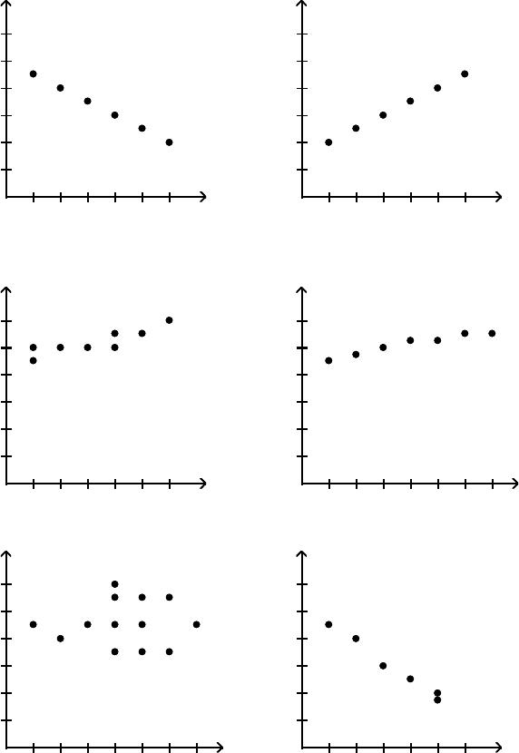
4) Whichscatterdiagramindicatesaperfectpositivecorrelation?
a
x
123456
y
12
10
8
6
4
2
x
123456
y
12
10
8
6
4
2
b
x
123456
y
12
10
8
6
4
2
x
123456
y
12
10
8
6
4
2
c
x
123456
y
12
10
8
6
4
2
x
123456
y
12
10
8
6
4
2
d
x
1234567
y
12
10
8
6
4
2
x
1234567
y
12
10
8
6
4
2
e
x
1234567
y
12
10
8
6
4
2
x
1234567
y
12
10
8
6
4
2
f
x
123456
y
12
10
8
6
4
2
x
123456
y
12
10
8
6
4
2
A)
b
B) a C) c D) f
Page93
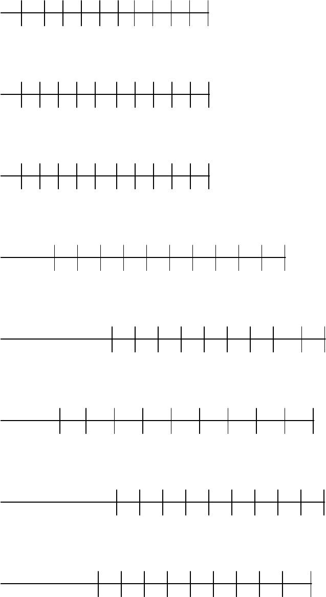
Thescatterdiagramshowstherelationshipbetweenaveragenumberofyearsofeducationandbirthsperwomanof
childbearingageinselectedcountries.Usethescatterplottodeterminewhetherthestatementistrueorfalse.
5) Thereisastrongpositivecorrelationbetweenyearsofeducationandbirthsperwoman.
BirthsperWoman
2468101214
10
9
8
7
6
5
4
3
2
1
2468101214
10
9
8
7
6
5
4
3
2
1
Averagenumberofyearsofeducation
ofMarriedWomenofChild–BearingAge
A) False B) True
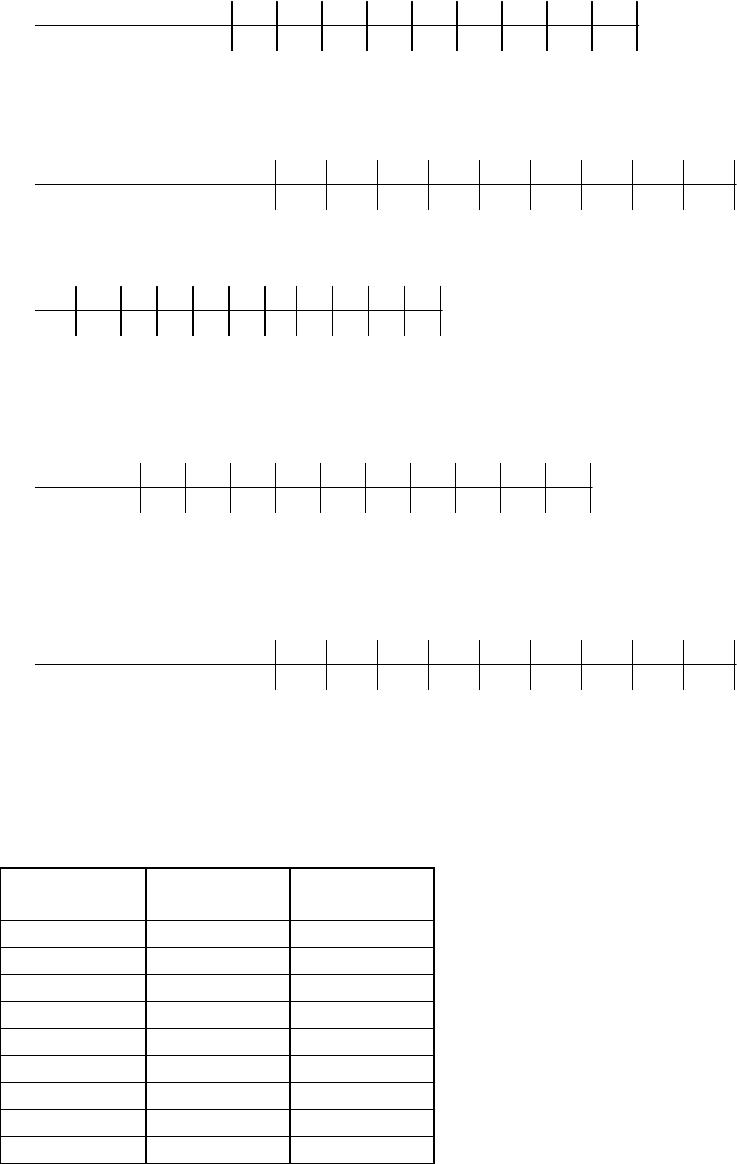
6) Thereisnocorrelationbetweenyearsofeducationandbirthsperwoman.
BirthsperWoman
2468101214
10
9
8
7
6
5
4
3
2
1
2468101214
10
9
8
7
6
5
4
3
2
1
Averagenumberofyearsofeducation
ofMarriedWomenofChild–BearingAge
A) False B) True
Page94
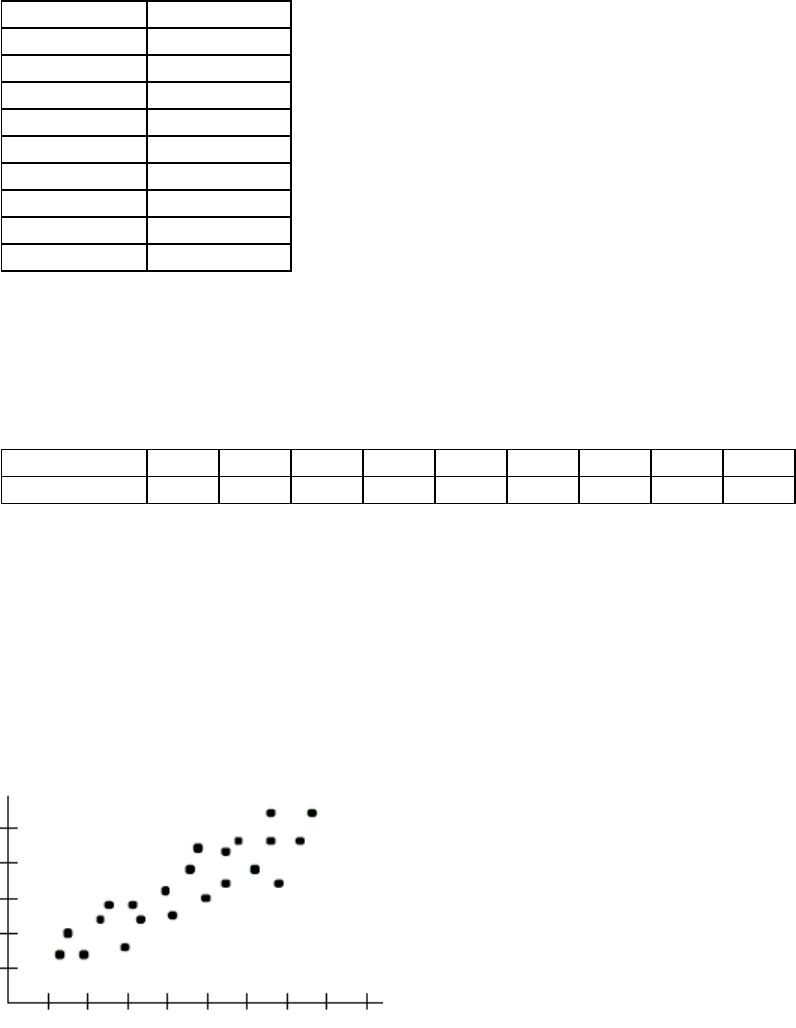
7) Thereisastrongnegativecorrelationbetweenyearsofeducationandbirthsperwoman.
BirthsperWoman
2468101214
10
9
8
7
6
5
4
3
2
1
2468101214
10
9
8
7
6
5
4
3
2
1
Averagenumberofyearsofeducation
ofMarriedWomenofChild–BearingAge
A) True B) False
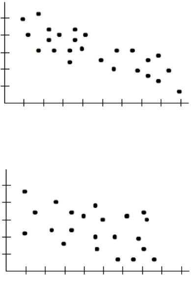
8) Thereisacausalrelationshipbetweenyearsofeducationandbirthsperwoman.
BirthsperWoman
2468101214
10
9
8
7
6
5
4
3
2
1
2468101214
10
9
8
7
6
5
4
3
2
1
Averagenumberofyearsofeducation
ofMarriedWomenofChild–BearingAge
A) False B) True
Page95
SHORTANSWER.Writethewordorphrasethatbestcompleteseachstatementoranswersthequestion.
Provideanappropriateresponse.
9) Constructascatterdiagramforthegivendata.Determinewhetherthereisapositivelinearcorrelation,
negativelinearcorrelation,ornolinearcorrelation.
x
y
–5
–10
–3
–8
4
9
1
1
–1
–2
–2
–6
0
–1
2
3
3
6
–4
–8
x
–6–5–4–3–2–1 123456
y
12
10
8
6
4
2
-2
-4
-6
-8
-10
-12
x
–6–5–4–3–2–1 123456
y
12
10
8
6
4
2
-2
-4
-6
-8
-10
-12
10) Constructascatterdiagramforthegivendata.Determinewhetherthereisapositivelinearcorrelation,
negativelinearcorrelation,ornolinearcorrelation.
x
y
–5
11
–3
6
4
–6
1
–1
–1
3
–2
4
0
1
2
–4
3
–5
–4
8
x
–6–5–4–3–2–1 123456
y
12
10
8
6
4
2
-2
-4
-6
-8
-10
-12
x
–6–5–4–3–2–1 123456
y
12
10
8
6
4
2
-2
-4
-6
-8
-10
-12
Page96
11) Constructascatterdiagramforthegivendata.Determinewhetherthereisapositivelinearcorrelation,
negativelinearcorrelation,ornolinearcorrelation.
x
y
–5
11
–3
–6
4
8
1
–3
–1
–2
–2
1
0
5
2
–5
3
6
–4
7
x
–6–5–4–3–2–1 123456
y
12
10
8
6
4
2
-2
-4
-6
-8
-10
-12
x
–6–5–4–3–2–1 123456
y
12
10
8
6
4
2
-2
-4
-6
-8
-10
-12
12) ThenumbersofhomerunsthatMarkMcGwirehitinthefirst13yearsofhismajorleaguebaseballcareerare
listedbelow.(Source:MajorLeagueHandbook)Constructascatterdiagramforthedata.Istherearelationship
betweenthehomerunsandthebattingaverages?
HomeRuns
BattingAverage
33 39 22 42 9939 52 58 70
.231 .235 .201 .268 .33 .252 .274 .312 .274 .299
x
15 30 45 60 75
y
0.35
0.3
0.25
0.2
0.15
x
15 30 45 60 75
y
0.35
0.3
0.25
0.2
0.15
Page97
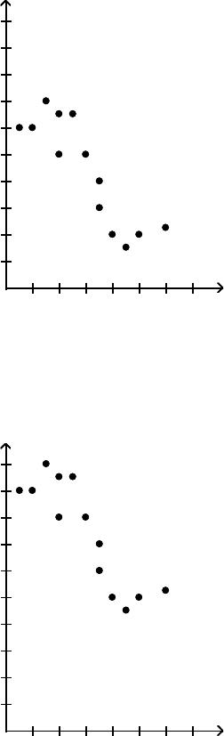
13) Thedatabelowrepresentthenumbersofabsencesandthefinalgradesof15randomlyselectedstudentsfrom
anastronomyclass.Constructascatterdiagramforthedata.Doyoudetectatrend?
Student Number
ofAbsences
FinalGrade
asaPercent
15 79
26 78
32 86
412 56
59 75
65 90
78 78
815 48
90 92
10 1 78
11 9 81
12 3 86
13 10 75
14 3 89
15 11 65
x
51015
y
100
90
80
70
60
50
40
x
51015
y
100
90
80
70
60
50
40
MULTIPLECHOICE.Choosetheonealternativethatbestcompletesthestatementoranswersthequestion.
14) Aresearcherdeterminesthatthelinearcorrelationcoefficientis0.85forapaireddataset.Thisindicatesthat
thereis
A) astrongpositivelinearcorrelation.
B) astrongnegativelinearcorrelation.
C) nolinearcorrelationbutthattheremaybesomeotherrelationship.
D) insufficientevidencetomakeanydecisionaboutthecorrelationofthedata.
15) Aninstructorwishestodetermineifthereisarelationshipbetweenthenumberofabsencesfromhisclassand
astudentʹsfinalgradeinthecourse.Whatisthepredictorvariable?
A) Absences B) FinalGrade
C) Theinstructorʹspointscaleforattendance D) Studentʹsperformanceonthefinalexamination
16) Amedicalresearcherwishestodetermineifthereisarelationshipbetweenthenumberofprescriptionswritten
bymedicalprofessionals,per100,childrenandthechildʹsage.Shesurveysallthepediatricianʹsina
geographicalregiontocollectherdata.Whatistheresponsevariable?
A) Ageofthechild B) Numberofprescriptionswritten
C) Pediatricianssurveyed D) 100prescriptions
17) TrueorFalse:Adoctorwishestodeterminetherelationshipbetweenamaleʹsageandthatmaleʹstotal
cholesterollevel.Hetests200malesandrecordseachmaleʹsageandthatmaleʹstotalcholesterollevel.The
malescholesterollevelisthepredictorvariable?
A) False B) True
18) Ascatterdiagramlocatesapointinatwodimensionalplane.Thediagramlocatesthe
variableonthehorizontalaxisandthe variableontheverticalaxis.
A) predictor;response B) response;predictor
C) response;study D) study;predictor
Page98
19) Ahistoryinstructorhasgiventhesamepretestandthesamefinalexaminationeachsemester.Heisinterested
indeterminingifthereisarelationshipbetweenthescoresofthetwotests.Hecomputesthelinearcorrelation
coefficientandnotesthatitis1.15.Whatdoesthiscorrelationcoefficientvaluetelltheinstructor?
A) Thehistoryinstructorhasmadeacomputationalerror.
B) Thereisastrongpositivecorrelationbetweenthetests.
C) Thereisastrongnegativecorrelationbetweenthetests.
D) Thecorrelationissomethingotherthanlinear.
20) Atrafficofficeriscompilinginformationabouttherelationshipbetweenthehourorthedayandthespeedover
thelimitatwhichthemotorististicketed.Hecomputesacorrelationcoefficientof0.12.Whatdoesthistell
theofficer?
A) Thereisaweakpositivelinearcorrelation.
B) Thereisamoderatepositivelinearcorrelation.
C) Thereisamoderatenegativelinearcorrelation.
D) Thereisinsufficientevidencetomakeanyconclusionsabouttherelationshipbetweenthevariables.
3 Computeandinterpretthelinearcorrelationcoefficient.
MULTIPLECHOICE.Choosetheonealternativethatbestcompletesthestatementoranswersthequestion.
Provideanappropriateresponse.
1) Calculatethelinearcorrelationcoefficientforthedatabelow.
x
y
–13
–12
–11
–10
–4
7
–7
–1
–9
–4
–10
–8
–8
–3
–6
1
–5
4
–12
–10
A) 0.990 B) 0.881 C) 0.819 D) 0.792
2) Calculatethelinearcorrelationcoefficientforthedatabelow.
x
y
–2
15
0
10
7
–2
4
3
2
7
1
8
3
5
5
0
6
–1
–1
12
A) –0.995 B) –0.671 C) –0.778 D) –0.885
3) Calculatethelinearcorrelationcoefficientforthedatabelow.
x
y
–9
16
–7
–1
0
13
–3
2
–5
3
–6
6
–4
10
–2
0
–1
11
–8
12
A) –0.104 B) –0.132 C) –0.549 D) –0.581
4) Thedatabelowarethefinalexamscoresof10randomlyselectedcalculusstudentsandthenumberofhours
theysleptthenightbeforetheexam.Calculatethelinearcorrelationcoefficient.
Hours,x
Scores,y
4
74
6
89
3
69
9
97
3
75
5
87
5
94
6
99
7
99
4
80
A) 0.847 B) 0.991 C) 0.761 D) 0.654
5) Thedatabelowaretheaverageone–waycommutetimes(inminutes)ofselectedstudentsduringasummer
literatureclassandthenumberofabsencesforthosestudentsfortheterm.Calculatethelinearcorrelation
coefficient.
Commutetime(min),x
Numberofabsences,y
71
–1
84
3
90
6
89
6
87
4
97
11
74
0
99
11
79
1
A) 0.980 B) 0.890 C) 0.881 D) 0.819
6) Thedatabelowaretheagesandannualpharmacybills(indollars)of9randomlyselectedemployees.
Calculatethelinearcorrelationcoefficient.
Age,x
Pharmacybill($),y
31
111
34
115
38
118
41
126
44
137
46
140
50
143
54
145
58
147
A) 0.960 B) 0.998 C) 0.890 D) 0.908
Page99
7) Thedatabelowarethenumberofhoursworked(perweek)andthefinalgradesof9randomlyselected
studentsfromadramaclass.Calculatethelinearcorrelationcoefficient.
Hoursworked,x
FinalGrade,y
3
91
6
79
9
73
7
75
12
64
5
85
18
48
11
69
8
75
A) –0.991 B) –0.888 C) –0.918 D) –0.899
8) Amanagerwishestodeterminetherelationshipbetweenthenumberofyearsthemanagerʹssales
representativeshavebeenwiththecompanyandtheiraveragemonthlysales(inthousandsofdollars).
Calculatethelinearcorrelationcoefficient.
Yearswithcompany,x
Sales,y
2
36
3
38
10
83
7
67
8
70
15
66
3
53
1
60
11
125
A) 0.632 B) 0.561 C) 0.717 D) 0.791
9) Inorderforacompanyʹsemployeestoworkinaforeignoffice,theymusttakeatestinthelanguageofthe
countrywheretheyplantowork.Thedatabelowshowstherelationshipbetweenthenumberofyearsthat
employeeshavestudiedaparticularlanguageandthegradestheyreceivedontheproficiencyexam.Calculate
thelinearcorrelationcoefficient.
Numberofyears,x
Gradesontest,y
7
62
8
69
8
76
9
83
7
74
10
91
6
59
11
94
7
73
A) 0.934 B) 0.911 C) 0.891 D) 0.902
10) InanareaoftheGreatPlains,recordswerekeptontherelationshipbetweentherainfall(ininches)andthe
yieldofwheat(bushelsperacre).Calculatethelinearcorrelationcoefficient.
Rainfall(ininches),x
Yield(bushelsperacre),y
9.8
48.5
8.1
44.2
12.7
56.8
11.8
57
18.1
80.4
9.6
47.2
6.3
29.9
14.9
74
15.3
76.8
A) 0.981 B) 0.998 C) 0.900 D) 0.899
SHORTANSWER.Writethewordorphrasethatbestcompleteseachstatementoranswersthequestion.
11) Calculatethecoefficientofcorrelation,r,lettingRow1representthex–valuesandRow2representthe
y–values.Nowcalculatethecoefficientofcorrelation,r,lettingRow2representthex–valuesandRow1
representthey–values.Whateffectdoesswitchingtheexplanatoryandresponsevariableshaveonthelinear
correlationcoefficient?
Row1
Row2
–10
0
–8
18
–1
19
–4
11
–6
8
–7
4
–5
9
–3
13
–2
16
–9
18
4 Determinewhetheralinearrelationexistsbetweentwovariables.
MULTIPLECHOICE.Choosetheonealternativethatbestcompletesthestatementoranswersthequestion.
Computethelinearcorrelationcoefficientbetweenthetwovariablesanddeterminewhetheralinearrelationexists.
1) x23556
y1.3 1.6 2.1 2.2 2.7
A) r=0.983;linearrelationexists B) r=0.983;nolinearrelationexists
C) r=0.883;linearrelationexists D) r=0.883;nolinearrelationexists
2) x2411 8657910 3
y0219 11 84913 16 2
A) r=0.990;linearrelationexists B) r=0.881;nolinearrelationexists
C) r=0.819;linearrelationexists D) r=0.792;nolinearrelationexists
3) x–11 –9–2–5–7–8–6–4–3–10
y19 14 2711 12 94316
A) r=–0.995;linearrelationexists B) r= –0.995;nolinearrelationexists
C) r=–0.885;nolinearrelationexists D) r= –0.885;linearrelationexists
Page100
4) x923425910
y85 52 55 68 67 86 83 73
A) r=0.708;linearrelationexists B) r=0.235;nolinearrelationexists
C) r=–0.708;linearrelationexists D) r=0.708;nolinearrelationexists
5) x10 11 16 9715 16 10
y96 51 62 58 89 81 46 51
A) r=–0.335;nolinearrelationexists B) r=0.462;linearrelationexists
C) r=–0.335;linearrelationexists D) r= –0.284;nolinearrelationexists
6) Thetablebelowshowsthescoresonanend–of–yearprojectof10randomlyselectedarchitecturestudentsand
thenumberofdayseachstudentspentworkingontheproject.
Days,x
Score,y
5
73
7
88
4
68
10
96
4
74
6
86
6
93
7
98
8
98
5
79
A) r=0.847;linearrelationexists B) r=0.847;nolinearrelationexists
C) r=0.761;linearrelationexists D) r=0.761;nolinearrelationexists
7) Thetablebelowshowstheagesandweights(inpounds)of9randomlyselectedtenniscoaches.
Age,x
Weight(pounds),y
36
112
39
116
43
119
46
127
49
138
51
141
55
144
59
146
63
148
A) r=0.960;linearrelationexists B) r=0.960;nolinearrelationexists
C) r=0.908;nolinearrelationexists D) r=0.908;linearrelationexists
8) Thetableshowsthenumberofdaysofflastyearandtheearningsfortheyear(inthousandsofdollars)fornine
randomlyselectedinsurancesalesmen.
Numberofdaysoff,x
Earningsfortheyear(thousandsofdollars),y
0
97
3
85
6
79
4
81
9
70
2
91
15
54
8
75
5
81
A) r=–0.991;linearrelationexists B) r= –0.991;nolinearrelationexists
C) r=–0.899;linearrelationexists D) r= –0.899;nolinearrelationexists
9) Amanagerwishestodeterminewhetherthereisarelationshipbetweenthenumberofyearshersales
representativeshavebeenwiththecompanyandtheiraveragemonthlysales.Thetableshowstheyearsof
serviceforeachofhersalesrepresentativesandtheiraveragemonthlysales(inthousandsofdollars).
Yearswithcompany,x6 714 11 12 19 7515
Sales,y36 38 83 67 70 66 53 60 125
A) r=0.632;nolinearrelationexists B) r=0.632;linearrelationexists
C) r=0.717;linearrelationexists D) r=0.717;nolinearrelationexists
10) Toinvestigatetherelationshipbetweenyieldofsoybeansandtheamountoffertilizerused,aresearcher
dividesafieldintoeightplotsofequalsizeandappliesadifferentamountoffertilizertoeachplot.Thetable
showstheyieldofsoybeansandtheamountoffertilizerusedforeachplot.
Amountoffertilizer(pounds),x 11.5 22.5 33.5 44.5
Yieldofsoybeans(pounds),y25 21 27 28 36 35 32 34
A) r=0.819;linearrelationexists B) r=0.729;nolinearrelationexists
C) r=0.683;linearrelationexists D) r=0.683;nolinearrelationexists
5 Explainthedifferencebetweencorrelationandcausation.
MULTIPLECHOICE.Choosetheonealternativethatbestcompletesthestatementoranswersthequestion.
Provideanappropriateresponse.
1) Avariablethatisrelatedtoeithertheresponsevariableorthepredictorvariableorboth,butwhichisexcluded
fromtheanalysisisa
A) lurkingvariable. B) randomvariable.
C) discretevariable. D) qualitativevariable.
Page101
SHORTANSWER.Writethewordorphrasethatbestcompleteseachstatementoranswersthequestion.
2) Forarandomsampleof100Americancities,thelinearcorrelationcoefficientbetweenthenumberofrobberies
lastyearandthenumberofschoolsinthecitywasfoundtober=0.725.Whatdoesthisimply?Doesthis
suggestthatbuildingmoreschoolsinacitycouldleadtomorerobberies?Whyorwhynot?Whatisalikely
lurkingvariable?
3) Forarandomsampleof30countries,thelinearcorrelationcoefficientbetweentheinfantmortalityrateandthe
averagenumberofcarspercapitawasfoundtober=–0.717.Whatdoesthisimply?Doesthissuggestthatif
peoplebuymorecars,thiscouldlowertheinfantmortalityrate?Whyorwhynot?Whatisalikelylurking
variable?
4) Arandomsampleof200menagedbetween20and60wasselectedfromacertaincity.Thelinearcorrelation
coefficientbetweenincomeandbloodpressurewasfoundtober=0.807.Whatdoesthisimply?Doesthis
suggestthatifamangetsasalaryraisehisbloodpressureislikelytorise?Whyorwhynot?Whatarelikely
lurkingvariables?
4.2 Least–SquaresRegression
1 Findtheleast–squaresregressionlineandusethelinetomakepredictions.
MULTIPLECHOICE.Choosetheonealternativethatbestcompletesthestatementoranswersthequestion.
Provideanappropriateresponse.
1) Findtheequationoftheregressionlineforthegivendata.Roundvaluestothenearestthousandth.
x
y
–5
–10
–3
–8
4
9
1
1
–1
–2
–2
–6
0
–1
2
3
3
6
–4
–8
A) y
^
=2.097x–0.552 B) y
^
=0.522x–2.097
C) y
^
=2.097x+0.552 D) y
^
=–0.552x+2.097
2) Findtheequationoftheregressionlineforthegivendata.Roundvaluestothenearestthousandth.
x
y
–5
11
–3
6
4
–6
1
–1
–1
3
–2
4
0
1
2
–4
3
–5
–4
8
A) y
^
=–1.885x+0.758 B) y
^
=0.758x+1.885 C) y
^
=–0.758x–1.885 D) y
^
=1.885x–0.758
3) Findtheequationoftheregressionlineforthegivendata.Roundvaluestothenearestthousandth.
x
y
–5
11
–3
–6
4
8
1
–3
–1
–2
–2
1
0
5
2
–5
3
6
–4
7
A) y
^
=–0.206x+2.097 B) y
^
=2.097x–0.206 C) y
^
=0.206x–2.097 D) y
^
=–2.097x+0.206
4) Thedatabelowarethefinalexamscoresof10randomlyselectedhistorystudentsandthenumberofhours
theysleptthenightbeforetheexam.Findtheequationoftheregressionlineforthegivendata.Whatwouldbe
thepredictedscoreforahistorystudentwhoslept7hoursthepreviousnight?Isthisareasonablequestion?
Roundtheregressionlinevaluestothenearesthundredth,androundthepredictedscoretothenearestwhole
number.
Hours,x
Scores,y
3
65
5
80
2
60
8
88
2
66
4
78
4
85
5
90
6
90
3
71
A) y
^
=5.04x+56.11;91;Yes,itisreasonable.
B) y
^
=5.04x+56.11;91;No,itisnotreasonable.7hoursiswelloutsidethescopeofthemodel.
C) y
^
=–5.04x+56.11;21;No,itisnotreasonable.7hoursiswelloutsidethescopeofthemodel.
D) y
^
=–5.04x+56.11;21;Yes,itisreasonable.
Page102
5) Thedatabelowarethefinalexamscoresof10randomlyselectedhistorystudentsandthenumberofhours
theysleptthenightbeforetheexam.Findtheequationoftheregressionlineforthegivendata.Whatwouldbe
thepredictedscoreforahistorystudentwhoslept15hoursthepreviousnight?Isthisareasonablequestion?
Roundyourpredictedscoretothenearestwholenumber.Roundtheregressionlinevaluestothenearest
hundredth.
Hours,x
Scores,y
3
65
5
80
2
60
8
88
2
66
4
78
4
85
5
90
6
90
3
71
A) y
^
=5.04x+56.11;132;No,itisnotreasonable.15hoursiswelloutsidethescopeofthemodel.
B) y
^
=5.04x+56.11;132;Yes,itisreasonable.
C) y
^
=–5.04x+56.11;–20;No,itisnotreasonable.
D) y
^
=–5.04x+56.11;–20;Yes,itisreasonable.
6) Thedatabelowaretheaverageone–waycommutetimes(inminutes)forselectedstudentsandthenumberof
absencesforthosestudentsduringtheterm.Findtheequationoftheregressionlineforthegivendata.What
wouldbethepredictednumberofabsencesifthecommutetimewas95minutes?Isthisareasonablequestion?
Roundthepredictednumberofabsencestothenearestwholenumber.Roundtheregressionlinevaluestothe
nearesthundredth.
Commutetime(min),x
Numberofabsences,y
72
3
85
7
91
10
90
10
88
8
98
15
75
4
100
15
80
5
A) y
^
=0.45x–30.27;12absences;Yes,itisreasonable.
B) y
^
=0.45x–30.27;12absences;No,itisnotreasonable.95minutesiswelloutsidethescopeofthemodel.
C) y
^
=0.45x+30.27;73absences;Yes,itisreasonable.
D) y
^
=0.45x+30.27;73absences;No,itisnotreasonable.95minutesiswelloutsidethescopeofthemodel.
7) Thedatabelowaretheaverageone–waycommutetimes(inminutes)forselectedstudentsandthenumberof
absencesforthosestudentsduringtheterm.Findtheequationoftheregressionlineforthegivendata.What
wouldbethepredictednumberofabsencesifthecommutetimewas40minutes?Isthisareasonablequestion?
Roundthepredictednumberofabsencestothenearestwholenumber.Roundtheregressionlinevaluestothe
nearesthundredth.
Commutetime(min),x
Numberofabsences,y
72
3
85
7
91
10
90
10
88
8
98
15
75
4
100
15
80
5
A) y
^
=0.45x–30.27;–12absences;No,itisnotreasonable.40minutesiswelloutsidethescopeofthemodel.
B) y
^
=0.45x–30.27;–12absences;Yes,itisreasonable.
C) y
^
=0.45x+30.27;48absences;Yes,itisreasonable.
D) y
^
=0.45x+30.27;48absences;No,itisnotreasonable.40minutesiswelloutsidethescopeofthemodel.
8) Thedatabelowareagesandsystolicbloodpressures(measuredinmillimetersofmercury)of9randomly
selectedadults.Findtheequationoftheregressionlineforthegivendata.Whatwouldbethepredicted
pressureiftheagewas60?Roundthepredictedpressuretothenearestwholenumber.Roundtheregression
linevaluestothenearesthundredth.
Age,x
Pressure,y
38
116
41
120
45
123
48
131
51
142
53
145
57
148
61
150
65
152
A) y
^
=1.49x+60.46;150mm B) y
^
=60.46x–1.49;3626mm
C) y
^
=1.49x–60.46;29mm D) y
^
=60.46x+1.49;3629mm
Page103
9) Thedatabelowarethenumberofabsencesandthefinalgradesof9randomlyselectedstudentsfroma
literatureclass.Findtheequationoftheregressionlineforthegivendata.Whatwouldbethepredictedfinal
gradeifastudentwasabsent14times?Roundtheregressionlinevaluestothenearesthundredth.Roundthe
predictedgradetothenearestwholenumber.
Numberofabsences,x
Finalgrade,y
0
98
3
86
6
80
4
82
9
71
2
92
15
55
8
76
5
82
A) y
^
=–2.75x+96.14;58 B) y
^
=96.14x–2.75;1343
C) y
^
=–2.75x–96.14;134.64 D) y
^
=–96.14x+2.75;1343
10) Amanagerwishestodeterminetherelationshipbetweenthenumberofmilestraveled(inhundredsofmiles)
byhersalesrepresentativesandtheiramountofsales(inthousandsofdollars)permonth.Findtheequationof
theregressionlineforthegivendata.Whatwouldbethepredictedsalesifthesalesrepresentativetraveled0
miles?Isthisreasonable?Whyorwhynot?Roundtheregressionlinevaluestothenearesthundredth.
Milestraveled,x
Sales,y
2
31
3
33
10
78
7
62
8
65
15
61
3
48
1
55
11
120
A) y
^
=3.53x+37.92;$37,920;No;itisnotreasonableforarepresentativetotravel0milesandhaveapositive
amountofsales.
B) y
^
=3.53x+37.92;$3792;No;itisnotreasonableforarepresentativetotravel0milesandhaveapositive
amountofsales.
C) y
^
=3.53x+37.92;$37,920;Yes,itisreasonable.
D) y
^
=37.92x+3.53;$3792;Yes,itisreasonable.
11) Amanagerwishestodeterminetherelationshipbetweenthenumberofyearshersalesrepresentativeshave
beenemployedbythefirmandtheiramountofsales(inthousandsofdollars)permonth.Findtheequationof
theregressionlineforthegivendata.Whatwouldbethepredictedsalesifthesalesrepresentativewas
employedbythefirmfor30yearsIsthisreasonable?Whyorwhynot?Roundtheregressionlinevaluestothe
nearesthundredth.
Yearsemployed,x
Sales,y
2
31
3
33
10
78
7
62
8
65
15
61
3
48
1
55
11
120
A) y
^
=3.53x+37.92;$143,820;No;itisnotreasonable.30yearsofemploymentiswelloutsidethescopeof
themodel.
B) y
^
=3.53x+37.92;$143,820;;Yes,itisreasonable.
C) y
^
=3.53x–37.92;$67,980;No;itisnotreasonable.30yearsofemploymentiswelloutsidethescopeofthe
model.
D) y
^
=3.53x–37.92;$67,980;Yes;itisreasonable.
12) Inorderforacompanyʹsemployeestoworkinaforeignoffice,theymusttakeatestinthelanguageofthe
countrywheretheyplantowork.Thedatabelowshowstherelationshipbetweenthenumberofyearsthat
employeeshavestudiedaparticularlanguageandthegradestheyreceivedontheproficiencyexam.Findthe
equationoftheregressionlineforthegivendata.Roundtheregressionlinevaluestothenearesthundredth.
Numberofyears,x
Gradesontest,y
3
61
4
68
4
75
5
82
3
73
6
90
2
58
7
93
3
72
A) y
^
=6.91x+46.26 B) y
^
=6.91x–46.26 C) y
^
=46.26x–6.91 D) y
^
=46.26x+6.91
Page104
13) InanareaoftheGreatPlains,recordswerekeptontherelationshipbetweentherainfall(ininches)andthe
yieldofwheat(bushelsperacre).Findtheequationoftheregressionlineforthegivendata.Roundthe
regressionlinevaluestothenearestthousandth.
Rainfall(ininches),x
Yield(bushelsperacre),y
10.5
50.5
8.8
46.2
13.4
58.8
12.5
59.0
18.8
82.4
10.3
49.2
7.0
31.9
15.6
76.0
16.0
78.8
A) y
^
=4.379x+4.267 B) y
^
=–4.379x+4.267 C) y
^
=4.267x+4.379 D) y
^
=4.267x–4.379
SHORTANSWER.Writethewordorphrasethatbestcompleteseachstatementoranswersthequestion.
14) FindtheequationoftheregressionlinebylettingRow1representthex–valuesandRow2representthe
y–values.NowfindtheequationoftheregressionlinelettingRow2representthex–valuesandRow1
representthey–values.Whateffectdoesswitchingtheexplanatoryandresponsevariableshaveonthe
regressionline?
Row1
Row2
–5
–10
–3
–8
4
9
1
1
–1
–2
–2
–6
0
–1
2
3
3
6
–4
–8
15) Isthenumberofgameswonbyamajorleaguebaseballteaminaseasonrelatedtotheteamʹsbattingaverage?
Datafrom14teamswerecollectedandthesummarystatisticsyield:
y=
∑1,134,x
∑=3.642,y2
∑=93,110,x2
∑=0.948622,andxy
∑=295.54
Findtheleastsquarespredictionequationforpredictingthenumberofgameswon,y,usingastraight–line
relationshipwiththeteamʹsbattingaverage,x.
16) Thetableshows,fortheyears1997–2012,themeanhourlywageforresidentsofthetownofPityMeandthe
meanweeklyrentpaidbytheresidents.
Year Meanweeklyrent
(dollars)
Meanhourlywage
(dollars)
Year Meanweeklyrent
(dollars)
Meanhourlywage
(dollars)
1997 57 10.38 2005 116 28.99
1998 59 10.89 2006 113 28.63
1999 62 11.96 2007 112 36.75
2000 63 12.46 2008 86 14.55
2001 86 17.72 2009 90 17.90
2002 119 28.07 2010 90 14.67
2003 131 35.24 2011 100 17.97
2004 122 31.87 2012 115 22.23
Summarystatisticsyield:SSxx=1222.2771,SSxy=3031.7125,SSyy=9144.9375,x=21.2675,and
y=95.0625.Findtheleastsquareslinethatusesmeanhourlywagetopredictmeanweeklyrent.Roundvalues
tothenearestten–thousandth.
MULTIPLECHOICE.Choosetheonealternativethatbestcompletesthestatementoranswersthequestion.
17) Aresidualisthedifferencebetween
A) theobservedvalueofyandthepredictedvalueofy.
B) theobservedvalueofxandthepredictedvalueofx.
C) theobservedvalueofyandthepredictedvalueofx.
D) theobservedvalueofxandthepredictedvalueofy.
18) Theleastsquaresregressionline
A) minimizesthesumoftheresidualssquared.
B) maximizesthesumoftheresidualssquared.
C) minimizesthemeandifferencebetweentheresidualssquared.
D) maximizesthemeandifferencebetweentheresidualssquared.
Page105

19) Foragivendataset,theequationoftheleastsquaresregressionlinewillalwayspassthrough
A) (x,y). B) everypointinthegivendataset.
C) atleasttwopointinthegivendataset. D) they–interceptandtheslope.
2 Interprettheslopeandthey–interceptoftheleast–squaresregressionline.
MULTIPLECHOICE.Choosetheonealternativethatbestcompletesthestatementoranswersthequestion.
Provideanappropriateresponse.
1) Acountyrealestateappraiserwantstodevelopastatisticalmodeltopredicttheappraisedvalueofhousesina
sectionofthecountycalledEastMeadow.Oneofthemanyvariablesthoughttobeanimportantpredictorof
appraisedvalueisthenumberofroomsinthehouse.Consequently,theappraiserdecidedtofitthesimple
linearregressionmodel,y
^=β0+β1x,wherey=appraisedvalueofthehouse(in$thousands)andx=number
ofrooms.Usingdatacollectedforasampleofn=74housesinEastMeadow,thefollowingresultswere
obtained:
y
^=74.80+20.86x
sβ=71.24,t=1.05(fortestingβ0)
sβ=2.63,t=7.49(fortestingβ1)
SSE=60,775,MSE=841,s=29,r2=.44
Rangeofthex–values:5–11
Rangeofthey–values:160–300
Giveapracticalinterpretationoftheestimateoftheslopeoftheleastsquaresline.
A) Foreachadditionalroominthehouse,weestimatetheappraisedvaluetoincrease$20
,
860.
B) Foreachadditionalroominthehouse,weestimatetheappraisedvaluetoincrease$74,800.
C) Foreachadditionaldollarofappraisedvalue,weestimatethenumberofroomsinthehousetoincrease
by20.86rooms.
D) Forahousewith0rooms,weestimatetheappraisedvaluetobe$74,800.
2) Acountyrealestateappraiserwantstodevelopastatisticalmodeltopredicttheappraisedvalueofhousesina
sectionofthecountycalledEastMeadow.Oneofthemanyvariablesthoughttobeanimportantpredictorof
appraisedvalueisthenumberofroomsinthehouse.Consequently,theappraiserdecidedtofitthesimple
linearregressionmodel,y
^=β0+β1x,wherey=appraisedvalueofthehouse(in$thousands)andx=number
ofrooms.Usingdatacollectedforasampleofn=74housesinEastMeadow,thefollowingresultswere
obtained:
y
^=74.80+19.72x
sβ=71.24,t=1.05(fortestingβ0)
sβ=2.63,t=7.49(fortestingβ1)
SSE=60,775,MSE=841,s=29,r2=0.44
Rangeofthex–values:5–11
Rangeofthey–values:160–300
Giveapracticalinterpretationoftheestimateofthey–interceptoftheleastsquaresline.
A) Thereisnopracticalinterpretation,sinceahousewith0roomsisnonsensical.
B) Foreachadditionalroominthehouse,weestimatetheappraisedvaluetoincrease$74,800.
C) Foreachadditionalroominthehouse,weestimatetheappraisedvaluetoincrease$19,720.
D) Weestimatethebaseappraisedvalueforanyhousetobe$74,800.
Page106
3) IstherearelationshipbetweentheraisesadministratorsatStateUniversityreceiveandtheirperformanceon
thejob?Afacultygroupwantstodeterminewhetherjobrating(x)isausefullinearpredictorofraise(y).
Consequently,thegroupconsideredthestraight–lineregressionmodel,y
^=β0+β1x.Usingthemethodofleast
squares,thefacultygroupobtainedthefollowingpredictionequation,y
^=14,000+2,000x.Interpretthe
estimatedslopeoftheline.
A) Fora1–pointincreaseinanadministratorʹsrating,weestimatetheadministratorʹsraisetoincrease
$2,000.
B) Fora1–pointincreaseinanadministratorʹsrating,weestimatetheadministratorʹsraisetodecrease
$2,000.
C) Foranadministratorwitharatingof1.0,weestimatehis/herraisetobe$2,000.
D) Fora$1increaseinanadministratorʹsraise,weestimatetheadministratorʹsratingtodecrease2,000
points.
4) IstherearelationshipbetweentheraisesadministratorsatStateUniversityreceiveandtheirperformanceon
thejob?Afacultygroupwantstodeterminewhetherjobrating(x)isausefullinearpredictorofraise(y).
Consequently,thegroupconsideredthestraight–lineregressionmodel,y
^=β0+β1x.Usingthemethodofleast
squares,thefacultygroupobtainedthefollowingpredictionequation,y
^=14,000+2,000x.
Interprettheestimatedy–interceptoftheline.
A) Foranadministratorwhoreceivesaratingofzero,weestimatehisorherraisetobe$14,000.
B) ThebaseadministratorraiseatStateUniversityis$14,000.
C) Fora1–pointincreaseinanadministratorʹsrating,weestimatetheadministratorʹsraisetoincrease
$14,000.
D) Thereisnopracticalinterpretation,sinceratingof0isnonsensicalandoutsidetherangeofthesample
data.
5) Alargenationalbankchargeslocalcompaniesforusingitsservices.Abankofficialreportedtheresultsofa
regressionanalysisdesignedtopredictthebankʹscharges(y),measuredindollarspermonth,forservices
renderedtolocalcompanies.Oneindependentvariableusedtopredictservicechargetoacompanyisthe
companyʹssalesrevenue(x),measuredinmillionsofdollars.Datafor21companieswhousethebankʹs
serviceswereusedtofitthemodel,y
^=β0+β1x.Theresultsofthesimplelinearregressionareprovidedbelow.
y
^=2,700+20x,s=65,2–tailedp–value=0.064(fortestingβ1)
Interprettheestimateofβ0,they–interceptoftheline.
A) Thereisnopracticalinterpretationsinceasalesrevenueof$0isanonsensicalvalue.
B) Allcompanieswillbechargedatleast$2,700bythebank.
C) About95%oftheobservedservicechargesfallwithin$2,700oftheleastsquaresline.
D) Forevery$1millionincreaseinsalesrevenue,weexpectaservicechargetoincrease$2,700.
Page107
6) Civilengineersoftenusethestraight–lineequation,y
^
=β0+β1x,tomodeltherelationshipbetweenthemean
shearstrengthofmasonryjointsandprecompressionstress,x.Totestthistheory,aseriesofstresstestswere
performedonsolidbricksarrangedintripletsandjoinedwithmortar.Theprecompressionstresswasvaried
foreachtripletandtheultimateshearloadjustbeforefailure(calledtheshearstrength)wasrecorded.The
stressresultsforn=7triplettestsisshownintheaccompanyingtablefollowedbyaSASprintoutofthe
regressionanalysis.
TripletTest 1234567
ShearStrength(tons),y1.00 2.18 2.24 2.41 2.59 2.82 3.06
Precomp.Stress(tons),x00.60 1.20 1.33 1.43 1.75 1.75
AnalysisofVariance
Sumof Mean
Source DF Squares Square FValue Prob>F
Model 1 2.39555 2.39555 47.732 0.0010
Error 5 0.25094 0.05019
CTotal 6 2.64649
RootMSE 0.22403 R–square 0.9052
DepMean 2.32857 AdjR–sq 0.8862
C.V. 9.62073
ParameterEstimates
Parameter Standard TforHO:
Variable DF Estimate Error Parameter=0 Prob>|T|
INTERCEP 1 1.191930 0.18503093 6.442 0.0013
X 1 0.987157 0.14288331 6.909 0.0010
Giveapracticalinterpretationoftheestimateoftheslopeoftheleastsquaresline.
A) Forevery1tonincreaseinprecompressionstress,weestimatetheshearstrengthofthejointtoincrease
by0.987ton.
B) Foratriplettestwithaprecompressionstressof1ton,weestimatetheshearstrengthofthejointtobe
0.987ton.
C) Forevery0.987tonincreaseinprecompressionstress,weestimatetheshearstrengthofthejointto
increaseby1ton.
D) Foratriplettestwithaprecompressionstressof0tons,weestimatetheshearstrengthofthejointtobe
1.19tons.
Page108
7) Civilengineersoftenusethestraight–lineequation,y
^
=β0+β1x,tomodeltherelationshipbetweenthemean
shearstrengthofmasonryjointsandprecompressionstress,x.Totestthistheory,aseriesofstresstestswere
performedonsolidbricksarrangedintripletsandjoinedwithmortar.Theprecompressionstresswasvaried
foreachtripletandtheultimateshearloadjustbeforefailure(calledtheshearstrength)wasrecorded.The
stressresultsforn=7triplettestsisshownintheaccompanyingtablefollowedbyaSASprintoutofthe
regressionanalysis.
TripletTest 1234567
ShearStrength,y
(tons)
1.00 2.18 2.24 2.41 2.59 2.82 3.06
Precomp.Stress,x
(tons)
00.60 1.20 1.33 1.43 1.75 1.75
AnalysisofVariance
Sumof Mean
Source DF Squares Square FValue Prob>F
Model 1 2.39555 2.39555 47.732 0.0010
Error 5 0.25094 0.05019
CTotal 6 2.64649
RootMSE 0.22403 R–square 0.9052
DepMean 2.32857 AdjR–sq 0.8862
C.V. 9.62073
ParameterEstimates
Parameter Standard TforHO:
Variable DF Estimate Error Parameter=0 Prob>|T|
INTERCEP 1 1.191930 0.18503093 6.442 0.0013
X 1 0.987157 0.14288331 6.909 0.0010
Giveapracticalinterpretationoftheestimateofthey–interceptoftheleastsquaresline.
A) Foratriplettestwithaprecompressionstressof0tons,weestimatetheshearstrengthofthejointtobe
1.19tons.
B) Forevery1tonincreaseinprecompressionstress,weestimatetheshearstrengthofthejointtoincrease
by0.987ton.
C) Thereisnopracticalinterpretationsinceatriplettestwithaprecompressionstressof0tonsisoutsidethe
rangeofthesampledata.
D) Foratriplettestwithaprecompressionstressof0tons,weestimatetheshearstrengthofthejointto
increase1.19tons.
Page109
8) EachyearanationallyrecognizedpublicationconductsitsʺSurveyofAmericaʹsBestGraduateand
ProfessionalSchools.ʺAnacademicadvisorwantstopredictthetypicalstartingsalaryofagraduateatatop
businessschoolusingGMATscoreoftheschoolasapredictorvariable.TotalGMATscoresrangefrom200to
800.AsimplelinearregressionofSALARYversusGMATusing25datapointsshownbelow.
β0
^=–92040β
^1=228s=3213R2=0.66r=0.81df=23t=6.67
Giveapracticalinterpretationofβ0
^=–92040.
A) ThevaluehasnopracticalinterpretationsinceaGMATof0isnonsensicalandoutsidetherangeofthe
sampledata.
B) WeexpecttopredictSALARYtowithin2(92040)=$184,080ofitstruevalueusingGMATina
straight–linemodel.
C) WeestimateSALARYtodecrease$92,040forevery1–pointincreaseinGMAT.
D) WeestimatethebaseSALARYofgraduatesofatopbusinessschooltobe$–92,040.
9) EachyearanationallyrecognizedpublicationconductsitsʺSurveyofAmericaʹsBestGraduateand
ProfessionalSchools.ʺAnacademicadvisorwantstopredictthetypicalstartingsalaryofagraduateatatop
businessschoolusingGMATscoreoftheschoolasapredictorvariable.TotalGMATscoresrangefrom200to
800.AsimplelinearregressionofSALARYversusGMATusing25datapointsshownbelow.
β0
^=–92040β
^1=228s=3213R2=0.66r=0.81df=23t=6.67
Giveapracticalinterpretationofβ1
^=228.
A) WeestimateSALARYtoincrease$228forevery1–pointincreaseinGMAT.
B) WeexpecttopredictSALARYtowithin2(228)=$456ofitstruevalueusingGMATinastraight–line
model.
C) WeestimateGMATtoincrease228pointsforevery$1increaseinSALARY.
D) ThevaluehasnopracticalinterpretationsinceaGMATof0isnonsensicalandoutsidetherangeofthe
sampledata.
10) Arealestatemagazinereportedtheresultsofaregressionanalysisdesignedtopredicttheprice(y),measured
indollars,ofresidentialpropertiesrecentlysoldinanorthernVirginiasubdivision.Oneindependentvariable
usedtopredictsalepriceisGLA,grosslivingarea(x),measuredinsquarefeet.Datafor157propertieswere
usedtofitthemodel,y
^=β0+β1x.Theresultsofthesimplelinearregressionareprovidedbelow.
y
^=96,600+22.5xs=6500r2=–0.77t=6.1(fortestingβ1)
Interprettheestimateofβ0,they–interceptoftheline.
A) Thereisnopracticalinterpretation,sinceagrosslivingareaof0isanonsensicalvalue.
B) AllresidentialpropertiesinVirginiawillsellforatleast$96,600.
C) About95%oftheobservedsalepricesfallwithin$96,600oftheleastsquaresline.
D) Forevery1–sqft.increaseinGLA,weexpectapropertyʹssalepricetoincrease$96,600.
Page110
SHORTANSWER.Writethewordorphrasethatbestcompleteseachstatementoranswersthequestion.
11) Inacomprehensiveroadtestonallnewcarmodels,onevariablemeasuredisthetimeittakesacarto
acceleratefrom0to60milesperhour.Tomodelaccelerationtime,aregressionanalysisisconductedona
randomsampleof129newcars.
TIME60:y=Elapsedtime(inseconds)from0mphto60mph
MAX:x1=Maximumspeedattained(milesperhour)
Initially,thesimplelinearmodelE(y)=β0+β1x1wasfittothedata.Computerprintoutsfortheanalysisare
givenbelow:
UNWEIGHTEDLEASTSQUARESLINEARREGRESSIONOFTIME60
PREDICTOR
VARIABLES COEFFICIENT STDERROR STUDENTʹSTP
CONSTANT 18.7171 0.63708 29.38 0.0000
MAX –0.08365 0.00491 –17.05 0.0000
R–SQUARED 0.6960 RESID.MEANSQUARE(MSE) 1.28695
ADJUSTEDR–SQUARED 0.6937 STANDARDDEVIATION 1.13444
SOURCE DF SS MS F P
REGRESSION 1374.285 374.285 290.83 0.0000
RESIDUAL 127 163.443 1.28695
TOTAL 128 537.728
CASESINCLUDED129MISSINGCASES0
Findandinterprettheestimateb1intheprintoutabove.
12) Inastudyoffeedingbehavior,zoologistsrecordedthenumberofgruntsofawarthogfeedingbyalakeinthe
15minuteperiodfollowingtheadditionoffood.Thedatashowingtheweeklynumberofgruntsandtheage
ofthewarthog(indays)arelistedbelow:
Week NumberofGrunts Age(days)
187 122
265 138
336 152
441 157
560 164
637 171
759 180
814 186
917 192
a.Writetheequationofastraight–linemodelrelatingnumberofgrunts(y)toage(x).
b.Givetheleastsquarespredictionequation.
c.Giveapracticalinterpretationofthevalueofβ0
^ifpossible.
d.Giveapracticalinterpretationofthevalueofβ1
^ifpossible.
Page111
MULTIPLECHOICE.Choosetheonealternativethatbestcompletesthestatementoranswersthequestion.
13) Giventhefollowingleastsquarespredictionequation,y
^
=–173+74x,weestimateyto by
witheach1–unitincreaseinx.
A) increase;74 B) decrease;74 C) decrease;173 D) increase;173
14) Giventheequationofaregressionlineisy
^
=3x–8,whatisthebestpredictedvalueforygivenx=2?
A) –2B)14C)13D)
–3
15) Giventheequationofaregressionlineisy
^
=–3.5x–2.6,whatisthebestpredictedvalueforygivenx=9.6?
A) –36.20 B) –31.00 C) 31.00 D) 36.20
16) Usetheregressionequationtopredictthevalueofyforx= –0.6.
x
y
–5
–10
–3
–8
4
9
1
1
–1
–2
–2
–6
0
–1
2
3
3
6
–4
–8
A) –1.810 B) –0.706 C) 2.428 D) 1.766
17) Usetheregressionequationtopredictthevalueofyforx=0.2.
x
y
–5
11
–3
6
4
–6
1
–1
–1
3
–2
4
0
1
2
–4
3
–5
–4
8
A) 0.381 B) 1.135 C) –1.733 D) 2.037
18) Thedatabelowarethefinalexamscoresof10randomlyselectedchemistrystudentsandthenumberofhours
theysleptthenightbeforetheexam.Whatisthebestpredictedvalueforygivenx=6?
Hours,x
Scores,y
3
65
5
80
2
60
8
88
2
66
4
78
4
85
5
90
6
90
3
71
A) 86 B) 85 C) 84 D) 87
19) Thedatabelowarethetemperaturesonrandomlychosendaysduringthesummerinonecityandthenumber
ofemployeeabsencesonthosedaysforacompanylocatedinthesamecity.Whatisthebestpredictedvalue
forygivenx=102?
Temperature,x
Numberofabsences,y
72
3
85
7
91
10
90
10
88
8
98
15
75
4
100
15
80
5
A) 16 B) 17 C) 18 D) 19
20) Thedatabelowaretheagesandsystolicbloodpressures(measuredinmillimetersofmercury)of9randomly
selectedadults.Whatisthebestpredictedvalueforygivenx=37?
Age,x
Pressure,y
38
116
41
120
45
123
48
131
51
142
53
145
57
148
61
150
65
152
A) 116 B) 118 C) 114 D) 112
21) Thedatabelowarethenumberofabsencesandthesalaries(inthousandsofdollars)of9randomlyselected
employeesfromanengineeringfirm.Whatisthebestpredictedvalueforygivenx=1?
.Numberofabsences,x
Salary,y
0
98
3
86
6
80
4
82
9
71
2
92
15
55
8
76
5
82
A) 93 B) 94 C) 95 D) 92
Page112
22) Inorderforacompanyʹsemployeestoworkfortheforeignoffice,theymusttakeatestinthelanguageofthe
countrywheretheyplantowork.Thedatabelowshowtherelationshipbetweenthenumberofyearsthat
employeeshavestudiedaparticularlanguageandthegradestheyreceivedontheproficiencyexam.Whatis
thebestpredictedvalueforygivenx=5.5?
Numberofyears,x
Gradesontest,y
3
61
4
68
4
75
5
82
3
73
6
90
2
58
7
93
3
72
A) 84 B) 82 C) 80 D) 86
23) InanareaoftheGreatPlains,recordswerekeptontherelationshipbetweentherainfall(ininches)andthe
yieldofwheat(bushelsperacre).Whichisthebestpredictedvalueforygivenx=15.6?
Rainfall(ininches),x
Yield(bushelsperacre),y
10.5
50.5
8.8
46.2
13.4
58.8
12.5
59.0
18.8
82.4
10.3
49.2
7.0
31.9
15.6
76.0
16.0
78.8
A) 72.6 B) 72.9 C) 72.4 D) 73.1
SHORTANSWER.Writethewordorphrasethatbestcompleteseachstatementoranswersthequestion.
24) Acalculusinstructorisinterestedinfindingthestrengthofarelationshipbetweenthefinalexamgradesof
studentsenrolledinCalculusIandCalculusIIathiscollege.Thedata(inpercentages)arelistedbelow.
CalculusI
CalculusII
88
81
78
80
62
55
75
78
95
90
91
90
83
81
86
80
98
100
a)Graphascatterdiagramofthedata.
b)Findanequationoftheregressionline.
c)PredictaCalculusIIexamscoreforastudentwhoreceivesan80inCalculusI.
MULTIPLECHOICE.Choosetheonealternativethatbestcompletesthestatementoranswersthequestion.
25) InoneareaofRussia,recordswerekeptontherelationshipbetweentherainfall(ininches)andtheyieldof
wheat(bushelsperacre).Thedatafora9yearperiodisasfollows:
RainFall,x13.1 11.4 16.0 15.1 21.4 12.9 9.6 18.2 18.6
Yield,y48.5 44.2 56.8 80.4 47.2 29.9 74.0 74.0 76.8
Theequationofthelineofleastsquaresisgivenasy
^=–9.12+4.38x.Howmanybushelsofwheatperacrecan
bepredictedifitisexpectedthattherewillbe17inchesofrain?
A) 65.34 B) 5.96 C) 61.18 D) 52.06
26) InanareaofRussia,recordswerekeptontherelationshipbetweentherainfall(ininches)andtheyieldof
wheat(bushelsperacre).Thedatafora9yearperiodisasfollows:
RainFall,x13.1 11.4 16.0 15.1 21.4 12.9 9.6 18.2 18.6
Yield,y48.5 44.2 56.8 80.4 47.2 29.9 74.0 74.0 76.8
Theequationofthelineofleastsquaresisgivenasy
^=–9.12+4.38x.Whatwouldbetheexpectednumberof
inchesofrainiftheyieldis60bushelsofwheatperacre?
A) 15.78 B) 253.68 C) 11.62 D) 64.74
27) InanareaofRussia,recordswerekeptontherelationshipbetweentherainfall(ininches)andtheyieldof
wheat(bushelsperacre).Thedatafora9yearperiodisasfollows:
RainFall,x13.1 11.4 16.0 15.1 21.4 12.9 9.6 18.2 18.6
Yield,y48.5 44.2 56.8 80.4 47.2 29.9 74.0 74.0 76.8
Theequationofthelineofleastsquaresisgivenasy
^=–9.12+4.38x.Howmanybushelsofwheatperacrecan
bepredictedifitisexpectedthattherewillbe30inchesofrain?
A) Cannotbecertainoftheresultbecause30inchesofrainexceedstheobserveddata.
B) 122.28
C) 140.52
D) 8.93
Page113
3 Computethesumofsquaredresiduals.
MULTIPLECHOICE.Choosetheonealternativethatbestcompletesthestatementoranswersthequestion.
Provideanappropriateresponse.
1) Theregressionlineforthegivendataisy
^
=2.097x–0.552.Determinetheresidualofadatapointforwhichx=
–1andy=–2.
x
y
–5
–10
–3
–8
4
9
1
1
–1
–2
–2
–6
0
–1
2
3
3
6
–4
–8
A) 0.649 B) –4.649 C) –2.649 D) 3.746
2) Theregressionlineforthegivendataisy
^
=–1.885x+0.758.Determinetheresidualofadatapointforwhichx
=1andy=–1.
x
y
–5
11
–3
6
4
–6
1
–1
–1
3
–2
4
0
1
2
–4
3
–5
–4
8
A) 0.127 B) –2.127 C) –1.127 D) –1.643
3) Theregressionlineforthegivendataisy
^
=–0.206x+2.097.Determinetheresidualofadatapointforwhichx
=2andy=–5.
x
y
–5
11
–3
–6
4
8
1
–3
–1
–2
–2
1
0
5
2
–5
3
6
–4
7
A) –6.685 B) –3.315 C) 1.685 D) –1.127
4) Theregressionlineforthegivendataisy
^
=5.044x+56.11.Determinetheresidualofadatapointforwhichx=
2andy=66.
Hours,x
Scores,y
3
65
5
80
2
60
8
88
2
66
4
78
4
85
5
90
6
90
3
71
A) –0.198 B) 132.198 C) 66.198 D) –387.014
5) Theregressionlineforthegivendataisy
^
=0.449x–30.27.Determinetheresidualofadatapointforwhichx=
85andy=7.
Temperature,x
Numberofabsences,y
72
3
85
7
91
10
90
10
88
8
98
15
75
4
100
15
80
5
A) –0.895 B) 14.895 C) 7.895 D) 112.127
6) Theregressionlineforthegivendataisy
^
=1.488x+60.46.Determinetheresidualofadatapointforwhichx=
53andy=145.
Age,x
Pressure,y
38
116
41
120
45
123
48
131
51
142
53
145
57
148
61
150
65
152
A) 5.676 B) 284.324 C) 139.324 D) –223.22
7) Theregressionlineforthegivendataisy
^
=–2.75x+96.14.Determinetheresidualofadatapointforwhichx=
8andy=76.
Numberofabsences,x
Finalgrade,y
0
98
3
86
6
80
4
82
9
71
2
92
15
55
8
76
5
82
A) 1.86 B) 150.14 C) 74.14 D) 120.86
8) Theregressionlineforthegivendataisy
^
=3.53x+37.92.Determinetheresidualofadatapointforwhichx=
3andy=33.
Yearsemployed,x
Sales,y
2
31
3
33
10
78
7
62
8
65
15
61
3
48
1
55
11
120
A) –15.51 B) 81.51 C) 48.51 D) –151.41
Page114
9) Theregressionlineforthegivendataisy
^
=6.91x+46.26.Determinetheresidualofadatapointforwhichx=4
andy=75.
Numberofyears,x
Gradesontest,y
3
61
4
68
4
75
5
82
3
73
6
90
2
58
7
93
3
72
A) 1.1 B) 148.9 C) 73.9 D) –560.51
10) Theregressionlineforthegivendataisy
^
=4.379x+4.267.Determinetheresidualofadatapointforwhichx=
13.4andy=58.8.
Rainfall(ininches),x
Yield(bushelsperacre),y
10.5
50.5
8.8
46.2
13.4
58.8
12.5
59.0
18.8
82.4
10.3
49.2
7.0
31.9
15.6
76.0
16.0
78.8
A) –4.1456 B) 121.7456 C) 62.9456 D) –248.3522
11) Computethesumofthesquaredresidualsoftheleast–squareslineforthegivendata.
x
y
–5
–10
–3
–8
4
9
1
1
–1
–2
–2
–6
0
–1
2
3
3
6
–4
–8
A) 7.624 B) 1.036 C) 2.097 D) 0
12) Thedatabelowarethefinalexamscoresof10randomlyselectedstatisticsstudentsandthenumberofhours
theysleptthenightbeforetheexam.Computethesumofthesquaredresidualsoftheleast –squareslineforthe
givendata.
Hours,x
Scores,y
3
65
5
80
2
60
8
88
2
66
4
78
4
85
5
90
6
90
3
71
A) 318.038 B) 804.062 C) 1122.1 D) 39.755
13) InanareaoftheGreatPlains,recordswerekeptontherelationshipbetweentherainfall(ininches)andthe
yieldofwheat(bushelsperacre).Computethesumofthesquaredresidualsoftheleast–squareslineforthe
givendata.
Rainfall(ininches),x
Yield(bushelsperacre),y
10.5
50.5
8.8
46.2
13.4
58.8
12.5
59.0
18.8
82.4
10.3
49.2
7.0
31.9
15.6
76.0
16.0
78.8
A) 87.192 B) 2207.628 C) 4.379 D) 0
14) Inastudyoffeedingbehavior,zoologistsrecordedthenumberofgruntsofawarthogfeedingbyalakeina15
minutetimeperiodfollowingtheadditionoffood.Thedatashowingtheweeklynumberofgruntsandtheage
ofthewarthog(indays)arelistedbelow.Computethesumofthesquaredresidualsoftheleastsquaredline
forthegivendata.
Week Numberof
Grunts
Age(days)
1 90 125
2 68 141
3 39 155
4 44 160
5 63 167
6 40 174
7 62 183
8 17 189
9 20 195
A) 5533.53 B) 188.84 C) 74.39 D) 13.74
Page115
15) Thedatabelowaretheagesandsystolicbloodpressure(measuredinMillimetersofmercury)of9randomly
selectedadults.
Age,x Pressure,y
38 116
41 12.
45 123
48 131
51 142
53 145
57 148
61 150
65 152
A) 123.63 B) 1.41 C) 1.99 D) 11.11
16) AcalculusinstructorisinterestedtheperformanceofhisstudentsfromCalculusIthatgoontoCalculusII.
Theirfinalgradesineachcourse(inpercent)aregivenbelow.Computethesumofthesquaredresidualsofthe
leastsquaredlineforthegivendata.
CalculusI88 78 62 75 95 91 83 86 98
CalculusII 81 80 55 78 90 90 81 80 100
A) 130.14 B) 30.85 C) 11.41 D) 1075.9
4.3 DiagnosticsontheLeast–SquaresRegressionLine
1 Computeandinterpretthecoefficientofdetermination.
MULTIPLECHOICE.Choosetheonealternativethatbestcompletesthestatementoranswersthequestion.
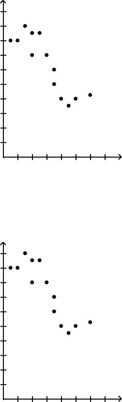
Choosethecoefficientofdeterminationthatmatchesthescatterplot.Assumethatthescalesonthehorizontaland
verticalaxesarethesame.
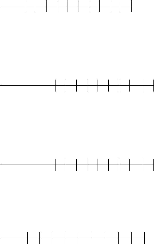
1) Response
Explanatory
A) R2=0.77 B) R2=0.38 C) R2=0.96 D) R2=0.51
Page116
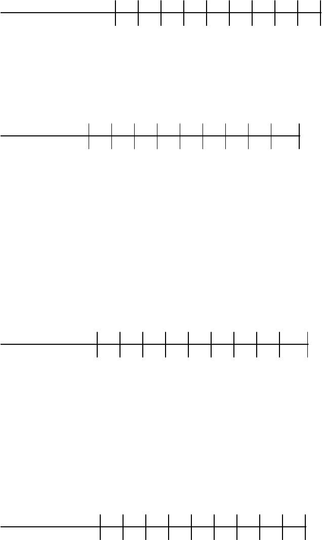
2) Response
Explanatory
A) R2=0.43 B) R2=–0.43 C) R2=0.82 D) R2=0.12
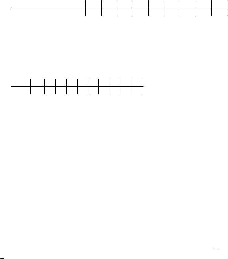
3) Response
Explanatory
A) R2=0.097 B) R2=–0.31 C) R2=0.76 D) R2=0.41
Usethelinearcorrelationcoefficientgiventodeterminethecoefficientofdetermination,R2.
4) r=0.66
A) R2=43.56% B) R2=81.24% C) R2=8.12% D) R2=4.356%
5) r=–0.11
A) R2=1.21% B) R2=33.17% C) R2=–1.21% D) R2=–33.17%
SHORTANSWER.Writethewordorphrasethatbestcompleteseachstatementoranswersthequestion.
Provideanappropriateresponse.
6) Calculatethecoefficientofdeterminationtothenearestthousandth,giventhatthelinearcorrelationcoefficient,
r,is0.837.Whatdoesthistellyouabouttheexplainedvariationandtheunexplainedvariationofthedata
abouttheregressionline?
7) Calculatethecoefficientofdeterminationtothenearestthousandth,giventhatthelinearcorrelationcoefficient,
r,is–0.625.Whatdoesthistellyouabouttheexplainedvariationandtheunexplainedvariationofthedata
abouttheregressionline?
8) Calculatethecoefficientofdetermination,giventhatthelinearcorrelationcoefficient,r,is1.Whatdoesthistell
youabouttheexplainedvariationandtheunexplainedvariationofthedataabouttheregressionline?
Page117
9) Inastudyoffeedingbehavior,zoologistsrecordedthenumberofgruntsofawarthogfeedingbyalakeinthe
15minuteperiodfollowingtheadditionoffood.Thedatashowingtheweeklynumberofgruntsandtheageof
thewarthog(indays)arelistedbelow.FindandinterpretthevalueofR2.RoundR2tothenearestthousandth.
NumberofGrunts Age(days)
87 122
65 138
36 152
41 157
60 164
37 171
59 180
14 186
17 192
MULTIPLECHOICE.Choosetheonealternativethatbestcompletesthestatementoranswersthequestion.
10) Inacomprehensiveroadtestonallnewcarmodels,onevariablemeasuredisthetimeittakesacarto
acceleratefrom0to60milesperhour.Tomodelaccelerationtime,aregressionanalysisisconductedona
randomsampleof129newcars.
TIME60: y=Elapsedtime(inseconds)from0mphto60mph
MAX: x1=Maximumspeedattained(milesperhour)
Initially,thesimplelinearmodelE(y)=β0+β1×1wasfittothedata.Computerprintoutsfortheanalysisare
givenbelow:
UNWEIGHTEDLEASTSQUARESLINEARREGRESSIONOFTIME60
PREDICTOR
VARIABLES COEFFICIENT STDERROR STUDENTʹSTP
CONSTANT 18.7171 0.63708 29.38 0.0000
MAX –0.08365 0.00491 –17.05 0.0000
R–SQUARED 0.6960 RESID.MEANSQUARE(MSE) 1.28695
ADJUSTEDR–SQUARED 0.6937 STANDARDDEVIATION 1.13444
SOURCE DF SS MS F P
REGRESSION 1374.285 374.285 290.83 0.0000
RESIDUAL 127 163.443 1.28695
TOTAL 128 537.728
CASESINCLUDED129MISSINGCASES0
Approximatelywhatpercentage,roundedtothenearestwholepercent,ofthesamplevariationinacceleration
timecanbeexplainedbythesimplelinearmodel?
A) 70% B) 0% C) –17% D) 8%
Page118
11) Amanufacturerofboilerdrumswantstouseregressiontopredictthenumberofman–hoursneededtoerect
drumsinthefuture.Themanufacturercollectedarandomsampleof35boilersandmeasuredthefollowing
twovariables:
MANHRS:y=Numberofman–hoursrequiredtoerectthedrum
PRESSURE:x1=Boilerdesignpressure(poundspersquareinch,i.e.,psi)
Initially,thesimplelinearmodelE(y)=β0+β1×1 wasfittothedata.Aprintoutfortheanalysisappearsbelow:
UNWEIGHTEDLEASTSQUARESLINEARREGRESSIONOFMANHRS
PREDICTOR
VARIABLES COEFFICIENT STDERROR STUDENTʹSTP
CONSTANT 1.88059 0.58380 3.22 0.0028
PRESSURE 0.00321 0.00163 2.17 0.0300
R–SQUARED 0.4342 RESID.MEANSQUARE(MSE) 4.25460
ADJUSTEDR–SQUARED 0.4176 STANDARDDEVIATION 2.06267
SOURCE DF SS MS F P
REGRESSION 1111.008 111.008 5.19 0.0300
RESIDUAL 34 144.656 4.25160
TOTAL 35 255.665
Giveapracticalinterpretationofthecoefficientofdetermination,R2.ExpressR2tothenearestwholepercent.
A) About43%ofthesamplevariationinnumberofman–hourscanbeexplainedbythesimplelinearmodel.
B) y
^
=1.88+0.00321xwillbecorrect43%ofthetime.
C) Manhoursneededtoerectdrumswillbeassociatedwithboilerdesignpressure43%ofthetime.
D) About2.06%ofthesamplevariationinnumberofman–hourscanbeexplainedbythesimplelinear
model.
Page119
12) Civilengineersoftenusethestraight–lineequation,E(y)=β0+β1x,tomodeltherelationshipbetweenthe
meanshearstrengthE(y)ofmasonryjointsandprecompressionstress,x.Totestthistheory,aseriesofstress
testswereperformedonsolidbricksarrangedintripletsandjoinedwithmortar.Theprecompressionstress
wasvariedforeachtripletandtheultimateshearloadjustbeforefailure(calledtheshearstrength)was
recorded.Thestressresultsforn=7triplettestsisshownintheaccompanyingtablefollowedbyaSAS
printoutoftheregressionanalysis.
TripletTest 1234567
ShearStrength(tons),y1.00 2.18 2.24 2.41 2.59 2.82 3.06
Precomp.Stress(tons),x00.60 1.20 1.33 1.43 1.75 1.75
AnalysisofVariance
Sumof Mean
Source DF Squares Square FValue Prob>F
Model 1 2.39555 2.39555 47.732 0.0010
Error 5 0.25094 0.05019
CTotal 6 2.64649
RootMSE 0.22403 R–square 0.9052
DepMean 2.32857 AdjR–sq 0.8862
C.V. 9.62073
ParameterEstimates
Parameter Standard TforHO:
Variable DF Estimate Error Parameter=0 Prob>|T|
INTERCEP 1 1.191930 0.18503093 6.442 0.0013
X 1 0.987157 0.14288331 6.909 0.0010
GiveapracticalinterpretationofR2,thecoefficientofdeterminationfortheleastsquaresmodel.ExpressR2to
thenearestwholepercent.
A) About91%ofthetotalvariationinthesampleofy–valuescanbeexplainedby(orattributedto)thelinear
relationshipbetweenshearstrengthandprecompressionstress.
B) Inrepeatedsampling,approximately91%ofallsimilarlyconstructedregressionlineswillaccurately
predictshearstrength.
C) Weexpecttopredicttheshearstrengthofatriplettesttowithinabout.91tonofitstruevalue.
D) Weexpectabout91%oftheobservedshearstrengthvaluestolieontheleastsquaresline.
13) ThedeanoftheBusinessSchoolatasmallFloridacollegewishestodeterminewhetherthegrade –point
average(GPA)ofagraduatingstudentcanbeusedtopredictthegraduateʹsstartingsalary.Morespecifically,
thedeanwantstoknowwhetherhigherGPAʹsleadtohigherstartingsalaries.Recordsfor23oflastyearʹs
BusinessSchoolgraduatesareselectedatrandom,anddataonGPA(x)andstartingsalary(y,in$thousands)
foreachgraduatewereusedtofitthemodel,E(y)=β0+β1x.Theresultsofthesimplelinearregressionare
providedbelow.
y
^=4.25+2.75x, SSxy=5.15,SSxx=1.87
SSyy=15.17,SSE=1.0075
Rangeofthex–values: 2.23–3.85
Rangeofthey–values: 9.3–15.6
CalculatethevalueofR2,thecoefficientofdetermination.
A) 0.934 B) 0.661 C) 0.872 D) 0.339
Page120
14) EachyearanationallyrecognizedpublicationconductsitsʺSurveyofAmericaʹsBestGraduateand
ProfessionalSchools.ʺAnacademicadvisorwantstopredictthetypicalstartingsalaryofagraduateatatop
businessschoolusingGMATscoreoftheschoolasapredictorvariable.AsimplelinearregressionofSALARY
versusGMATusing25datapointsshownbelow.
b0=–92040b1=228s=3213R2=0.66r=0.81df=23t=6.67
GiveapracticalinterpretationofR2=0.66.
A) 66%ofthesamplevariationinSALARYcanbeexplainedbyusingGMATinastraight –linemodel.
B) 66%ofthedifferencesinSALARYarecausedbydifferencesinGMATscores.
C) WeestimateSALARYtoincrease$.66forevery1–pointincreaseinGMAT.
D) WecanpredictSALARYcorrectly66%ofthetimeusingGMATinastraight –linemodel.
15) Arealestatemagazinereportedtheresultsofaregressionanalysisdesignedtopredicttheprice(y),measured
indollars,ofresidentialpropertiesrecentlysoldinanorthernVirginiasubdivision.Oneindependentvariable
usedtopredictsalepriceisGLA,grosslivingarea(x),measuredinsquarefeet.Datafor157propertieswere
usedtofitthemodel,E(y)=β0+β1x.Theresultsofthesimplelinearregressionareprovidedbelow.
y=96,600+22.5xs=6500R2=0.77t=6.1(fortestingβ1)
Interpretthevalueofthecoefficientofdetermination,R2.
A) 77%ofthetotalvariationinthesamplesalepricescanbeattributedtothelinearrelationshipbetween
GLA(x)and(y).
B) GLA(x)islinearlyrelatedtosaleprice(y)77%ofthetime.
C) 77%oftheobservedsaleprices(yʹs)willfallwithin2standarddeviationsoftheleastsquaresline.
D) Thereisamoderatelystrongpositivecorrelationbetweensaleprice(y)andGLA(x).
SHORTANSWER.Writethewordorphrasethatbestcompleteseachstatementoranswersthequestion.
16) Acompanykeepsextensiverecordsonitsnewsalespeopleonthepremisethatsalesshouldincreasewith
experience.Arandomsampleofsevennewsalespeopleproducedthedataonexperienceandsalesshownin
thetable.
MonthsonJob MonthlySales
y($thousands)
22.4
47.0
8 11.3
12 15.0
10.8
53.7
9 12.0
SummarystatisticsyieldSSxx=94.8571,SSxy=124.7571,SSyy=176.5171,x=5.8571,andy=7.4571.Findand
interpretthecoefficientofdetermination.RoundR2tothenearesthundredthofapercent.
17) Toinvestigatetherelationshipbetweenyieldofpotatoes,y,andleveloffertilizerapplication,x,an
experimenterdividesafieldintoeightplotsofequalsizeandappliesdifferingamountsoffertilizertoeach.
Theyieldofpotatoes(inpounds)andthefertilizerapplication(inpounds)arerecordedforeachplot.Thedata
areasfollows:
x11.5 2 2.5 3 3.5 4 4.5
y25 31 27 28 36 35 32 34
SummarystatisticsyieldSSxx=10.5,SSyy=112,andSSxy=25.Calculatethecoefficientofdetermination
roundedtothenearestten–thousandth.
Page121
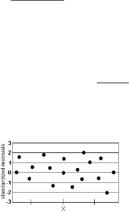
MULTIPLECHOICE.Choosetheonealternativethatbestcompletesthestatementoranswersthequestion.
18) Thecoefficientofcorrelationbetweenxandyisr=0.59.CalculatethecoefficientofdeterminationR2.Round
R2tothenearesthundredth.
A) 0.35 B) 0.59 C) 0.41 D) 0.65
SHORTANSWER.Writethewordorphrasethatbestcompleteseachstatementoranswersthequestion.
19) Thecoefficientofdeterminationforastraight–linemodelrelatingsellingpriceytomanufacturingcostxfora
particularitemisR2=0.83.Interpretthisvalue.
MULTIPLECHOICE.Choosetheonealternativethatbestcompletesthestatementoranswersthequestion.
20) Themeasuresthepercentageoftotalvariationintheresponsevariablethatisexplained
bytheleastsquaresregressionline.
A) coefficientofdetermination B) coefficientoflinearcorrelation
C) sumoftheresidualssquared D) slopeoftheregressionline
21) Ifthecoefficientofdeterminationiscloseto1,then
A) theleastsquaresregressionlineequationexplainsmostofthevariationintheresponsevariable.
B) theleastsquaresregressionlineequationhasnoexplanatoryvalue.
C) thesumofthesquareresidualsislargecomparedtothetotalvariation.
D) thelinearcorrelationcoefficientisclosetozero.
22) Thecoefficientofdeterminationistheofthelinearcorrelationcoefficient.
A) square B) squareroot C) opposite D) reciprocal
2 Performresidualanalysisonaregressionmodel.
MULTIPLECHOICE.Choosetheonealternativethatbestcompletesthestatementoranswersthequestion.
Analyzetheresiduallotbelow.Doesitviolateanyoftheconditionsforanadequatelinearmodel?
1)
A) No,theplotofresidualsisrandom.
B) Yes,thereisadiscernablepatternintheresiduals.
C) Yes,theresidualsdonotdisplayconstanterrorvariance.
Page122
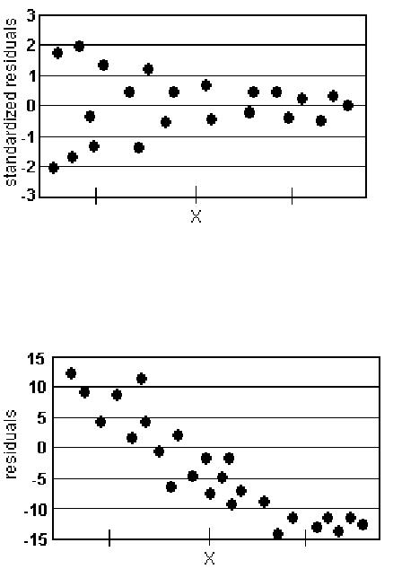
2)
A) Yes,theresidualsdonotdisplayconstanterrorvariance.
B) Yes,thereisadiscernablepatternintheresiduals.
C) No,theplotofresidualsisrandom.
3)
A) Yes,thereisadiscernablepatternintheresiduals.
B) Yes,theresidualsdonotdisplayconstanterrorvariance.
C) No,theplotofresidualsisrandom.
Provideanappropriateresponse.
4) TrueorFalse:Residualanalysiscannotbeusedtocheckforoutliers.
A) False B) True
5) TrueorFalse:Ifaresidualplotshowsanalmoststraightlinethenalinearmodelisappropriate.
A) False B) True
6) Todetermineifthereareoutliersinaleastsquaresregressionmodelʹsdataset,wecouldconstructaboxplotof
the
A) residuals. B) responsevariables.
C) predictorvariables. D) lurkingvariables.
Page123
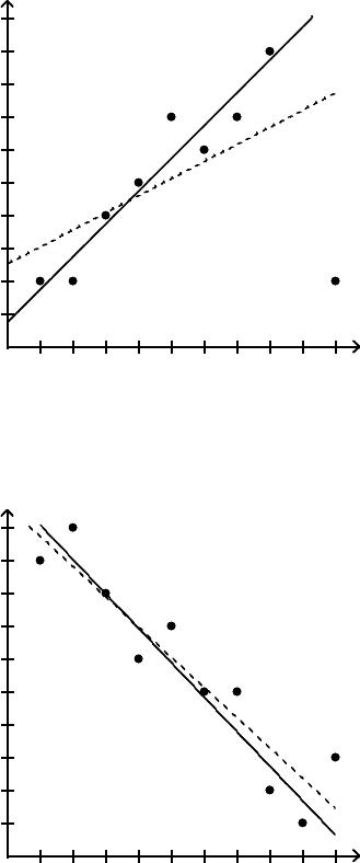
3 Identifyinfluentialobservations.
MULTIPLECHOICE.Choosetheonealternativethatbestcompletesthestatementoranswersthequestion.
AscatterdiagramisgivenwithoneofthepointslabeledʺA.ʺInaddition,therearetwoleast –squaresregressionlines
drawn.ThesolidlineexcludesthepointA.ThedashedlineincludesthepointA.Basedonthegraph,isthepointA
influential?
1)
x
12345678910
y
10
9
8
7
6
5
4
3
2
1
A
x
12345678910
y
10
9
8
7
6
5
4
3
2
1
A
A) yes B) no
2)
x
12345678910
y
10
9
8
7
6
5
4
3
2
1
A
x
12345678910
y
10
9
8
7
6
5
4
3
2
1
A
A) no B) yes
Provideanappropriateresponse.
3) Aninfluentialobservationisanobservationthatsignificantlyaffectsthevalueofthe
A) theslopeoftheleastsquaresregressionline. B) themeanoftheresponsevariable.
C) themedianofthepredictorvariable. D) themedianoftheresponsevariable.
4) Whateffectwillaninfluentialobservationhaveuponthegraphoftheleastsquaresregressionline?
A) Itwillpullthegraphtowardtheobservation.
B) Itwillhavenoeffect.
C) Itwillpushthegraphawayfromtheobservation.
D) Itwilllowerthevalueofthecorrelationcoefficienttomakefurtheranalysismeaningless.
Page124
4.4 ContingencyTablesandAssociation
1 Computethemarginaldistributionofavariable.
MULTIPLECHOICE.Choosetheonealternativethatbestcompletesthestatementoranswersthequestion.
Provideanappropriateresponse.
1) Thefollowingdatarepresentthelivingsituationofnewlywedsinalargemetropolitanareaandtheirannual
householdincome.Findthemarginalfrequencyfornewlywedswhorenttheirhome.
<$20,000 $20–35,000 $35–50,000 $50–75,000 >$75,000
Ownhome 31 52 202 355 524
Renthome 67 66 52 23 11
Livew/family 89 69 30 4 2
A) 219 B) 67 C) 11 D) 52
2) Thefollowingdatarepresentthelivingsituationofnewlywedsinalargemetropolitanareaandtheirannual
householdincome.Findthemarginalfrequencyfornewlywedswhomakebetween$20,000and$35,000per
year.
<$20,000 $20–35,000 $35–50,000 $50–75,000 >$75,000
Ownhome 31 52 202 355 524
Renthome 67 66 52 23 11
Livew/family 89 69 30 4 2
A) 187 B) 69 C) 52 D) 66
3) Thefollowingdatarepresentthelivingsituationofnewlywedsinalargemetropolitanareaandtheirannual
householdincome.Whatpercentofpeoplewhomakebetween$20,000and$35,000peryearowntheirown
home?Roundtothenearesttenthofapercent.
<$20,000 $20–35,000 $35–50,000 $50–75,000 >$75,000
Ownhome 31 52 202 355 524
Renthome 67 66 52 23 11
Livew/family 89 69 30 4 2
A) 27.8% B) 35.3% C) 36.9% D) 4.5%
4) Thefollowingdatarepresentthelivingsituationofnewlywedsinalargemetropolitanareaandtheirannual
householdincome.Whatpercentofpeoplewhoowntheirownhomemakebetween$35,000and$50,000per
year?Roundtothenearesttenthofapercent.
<$20,000 $20–35,000 $35–50,000 $50–75,000 >$75,000
Ownhome 31 52 202 355 524
Renthome 67 66 52 23 11
Livew/family 89 69 30 4 2
A) 17.4% B) 4.5% C) 30.5% D) 71.1%
Page125
5) Constructafrequencymarginaldistributionforthegivencontingencytable.
x1x2x3
y140 25 30
y265 60 60
A)
x1x2x3MarginalDistribution
y140 25 30 95
y265 60 60 185
MarginalDistribution 105 85 90 280
B)
x1x2x3MarginalDistribution
y140 25 30 95
y265 60 60 185
MarginalDistribution 105 85 90 560
C)
x1x2x3MarginalDistribution
y140 25 30 95
y265 60 60 185
MarginalDistribution 25 35 30 560
D)
x1x2x3MarginalDistribution
y140 25 30 105v
y265 60 60 85
MarginalDistribution 95 185 90 560
Page126

6) Constructarelativefrequencymarginaldistributionforthegivencontingencytable.Roundvaluesetothe
nearestthousandth.
x1x2x3
y120 25 25
y255 50 50
A)
x1x2x3
RelativeFrequency
MarginalDistribution
y120 25 25 0.311
y255 50 50 0.689
RelativeFrequency
MarginalDistribution 0.333 0.333 0.333 1
B)
x1x2x3
RelativeFrequency
MarginalDistribution
y120 25 25 0.311
y255 50 50 0.689
RelativeFrequency
MarginalDistribution 0.156 0.111 0.111 1
C)
x1x2x3
RelativeFrequency
MarginalDistribution
y120 25 25 0.70
y255 50 50 1.55
RelativeFrequency
MarginalDistribution 0.75 0.75 0.75 1
D)
RelativeFrequency
MarginalDistribution x1x2x3
y10.089 0.111 0.111
y20.244 0.222 0.222
Page127
7) Constructaconditionaldistributionbyxforthegivencontingencytable.Roundvaluesetothenearest
thousandth.
x1x2x3
y125 25 35
y275 75 70
A)
x1x2x3
y10.250 0.250 0.333
y20.750 0.750 0.667
Total 111
B)
x1x2x3
y10.250 0.250 0.333
y20.341 0.341 0.318
Total 111
C)
x1x2x3
y10.082 0.082 0.115
y20.246 0.246 0.230
D)
x1x2x3Total
y10.294 0.294 0.412 1
y20.341 0.341 0.318 1
8) Acontingencytablerelates
A) twocategoriesofdata.
B) thedifferenceinthemeansoftworandomvariables.
C) aparticularresponsewithorderinwhichthatresponseshouldbeapplied.
D) onlycontinuousrandomvariables.
9) Toeliminatetheeffectsofeithertheroworthecolumnvariablesinacontingencytable,a
distributioniscreated.
A) marginal B) normalized C) χ2D) Studentʹst
2 Usetheconditionaldistributiontoidentifyassociationamongcategoricaldata.
SHORTANSWER.Writethewordorphrasethatbestcompleteseachstatementoranswersthequestion.
Provideanappropriateresponse.
1) Thedatabelowshowtheageandfavoritetypeofmusicof779randomlyselectedpeople.Useα=0.05. What,if
any,associationexistsbetweenfavoritemusicandage?Discusstheassociation.
Age Country Rock Pop Classical
15–21 21 45 90 33
21–30 60 55 42 48
30–40 65 47 31 57
40–50 68 39 25 53
2) Thefollowingdatarepresentthelivingsituationofnewlywedsinalargemetropolitanareaandtheirannual
householdincome.What,ifany,associationexistsbetweenlivingsituationandhouseholdincome?Discussthe
association.
<$20,000 $20–35,000 $35–50,000 $50–75,000 >$75,000
Ownhome 31 52 202 355 524
Renthome 67 66 52 23 11
Livew/family 89 69 30 4 2
Page128
3 ExplainSimpsonʹsParadox.
SHORTANSWER.Writethewordorphrasethatbestcompleteseachstatementoranswersthequestion.
Provideanappropriateresponse.
1) Researchersconductedastudytodeterminewhichoftwodifferenttreatments,AorB,ismoreeffectiveinthe
treatmentofatherosclerosis.Theresultsoftheirexperimentaregiveninthetable.(a)Whichtreatmentappears
tobemoreeffective?Why?
TreatmentA TreatmentB
Effective 420 435
Noteffective 130 140
Thedatainthetabledonottakeintoaccounttheseriousnessofthecase.Thedatashowninthenexttable
showtheeffectivenessofeachtreatmentforbothmildandadvancedcasesofatherosclerosis.
Mild Advanced
atherosclerosis atherosclerosis
TreatmentATreatmentBTreatmentATreatmentB
Effective 31095 110340
Noteffective 8020 50120
(b)DeterminetheproportionofmildcasesofatherosclerosisthatwereeffectivelydealtwithusingtreatmentA.
DeterminetheproportionofmildcasesofatherosclerosisthatwereeffectivelydealtwithusingtreatmentB.
(c)Repeatpart(b)foradvancedcasesofatherosclerosistocreateaconditionaldistributionofeffectivenessby
treatmentforeachcategoryofthedisease.
(d)Writeashortreportdetailingandexplainingyourfindings.
2) Acompanyencouragesapplicationsfromminoritygroupswhotheyfeelareunder–representedinthe
company.Thetableshowsthenumberofapplicationsthatwereacceptedlastyearfrompeoplebelongingto
minoritygroupsandthenumberofapplicationsthatwereacceptedfrompeoplenotbelongingtominority
groups.Onlyapplicationsfromwellqualifiedapplicantsareincludedintheanalysis.(a)Doestheacceptance
rateappeartobehigherforthosebelongingtominoritygroupsorforthosenotbelongingtominoritygroups?
Why?
Minority Notminority
Accepted 70 79
Rejected 460 500
Thedatainthetabledonottakeintoaccountthedepartmentofthecompany.Thedatashowninthenexttable
showthenumberofapplicationsacceptedfromeachgroupwithineachdepartment.
DepartmentA DepartmentB DepartmentC
MinorityNotminority MinorityNotminority MinorityNotminority
Accepted 2710 2234 2135
Rejected 260110 80150 120240
(b)DeterminetheproportionofminorityapplicationsthatwereacceptedwithindepartmentA.Determinethe
proportionofnon–minorityapplicationsthatwereacceptedwithindepartmentA.
(c)Repeatpart(b)fordepartmentsBandCtocreateaconditionaldistributionofacceptanceratebygroupfor
eachdepartmentofthecompany.
(d)Writeashortreportdetailingandexplainingyourfindings.
Page129
4.5 NonlinearRegression:Transformations(onCD)
1 Convertbetweenexponentialandlogarithmicexpressions.
MULTIPLECHOICE.Choosetheonealternativethatbestcompletesthestatementoranswersthequestion.
Changetheexponentialexpressiontoanequivalentexpressioninvolvingalogarithm.
1) 23=8
A) log28=3 B) log82=3 C) log38=2 D) log23=8
2) 23=x
A) log2x=3 B) logx2=3 C) log3x=2 D) log23=x
3) 83=y
A) log8y=3 B) log3y=8 C) logy8=3 D) logy3=8
4) 7x=49
A) log749=x B) logx49 =7 C) log497=x D) log49x=7
5) 2x=279
A) log2279=x B) log2792=x C) log279x=2 D) log2x=279
Changethelogarithmicexpressiontoanequivalentexpressioninvolvinganexponent.
6) log39=2
A) 32=9B)2
3=9C)3
9=2D)9
2=3
7) log4x=3
A) 43=xB)3
4=xC)4
x=3D)x
3=4
8) logb32=5
A) b5=32 B) 5
b
=32 C) 325=bD)32
b
=5
9) log464=x
A) 4x=64 B) x4=64 C) 64x=4D)64
4=x
2 Simplifylogarithmicexpressions.
MULTIPLECHOICE.Choosetheonealternativethatbestcompletesthestatementoranswersthequestion.
Writetheexpressionasasumoflogs.Expresspowersasfactors.
1) log10xy
A) log10x+log10y B) log10x–log10y C) log5x+log5y D) log5x–log5y
2) log7x2
A) 2log7x B) 7log2xC)7logx D) 2log7x2
3) logbyz2
A) logby+2logbz B) 2logby+2logbz C) 2logbyz D) logby+logb2z
Page130
4) logby7z3
A) 7logby+3logbz B) 21logbyz C) logb(yz)21 D) logb21yz
Useacalculatortoevaluatetheexpression.Roundyouranswertothreedecimalplaces.
5) log111
A) 2.045 B) 4.710 C) 2.049 D) 2.041
6) log2.99
A) 0.476 B) 1.095 C) 0.490 D) 0.461
7) 101.4
A) 25.119 B) 31.623 C) 4.055 D) 39.811
8) 100.5826
A) 3.825 B) 0.261 C) 0.558 D) 1.144
3 Uselogarithmictransformationstolinearizeexponentialrelations.
SHORTANSWER.Writethewordorphrasethatbestcompleteseachstatementoranswersthequestion.
Provideanappropriateresponse.
1) Thefollowingdatarepresentthebacteriapopulationinalaboratoryexperiment.Theresearcherssuspectthat
thepopulationisgrowingexponentially.Determinethelogarithmofthey–valuessothatY=logy.
Day,x Population,y
0 1828
1 4982
2 13,494
3 36,784
4 100,058
5 272,152
MULTIPLECHOICE.Choosetheonealternativethatbestcompletesthestatementoranswersthequestion.
2) Thefollowingdatarepresentthebacteriapopulationinalaboratoryexperiment.Theresearcherssuspectthat
thepopulationisgrowingexponentially.Findtheexponentialequationofbestfit.
Day,x Population,y
0 1952
1 5319
2 14410
3 39279
4 106845
5 290613
A) y
^
=3.291+0.435x B) y
^
=3.458+1.151x
C) y
^
=–7.537+2.301x D) y
^
=–50,222.143+50,650.057x
Page131
4 Uselogarithmictransformationstolinearizepowerrelations.
SHORTANSWER.Writethewordorphrasethatbestcompleteseachstatementoranswersthequestion.
Provideanappropriateresponse.
1) Thefollowingdatarepresenttheperiods(inseconds)ofsimplependulumsofvariouslengths(infeet).
Determinethelogarithmofboththex–andy–valuessothatX=logxandY=logy.
Length,x Period,y
1 1.3
2 1.8
3 2.3
4 2.6
5 2.9
6 3.2
MULTIPLECHOICE.Choosetheonealternativethatbestcompletesthestatementoranswersthequestion.
2) Thefollowingdatarepresenttheperiods(inseconds)ofsimplependulumsofvariouslengths(infeet).Findthe
powerequationofbestfit.
Length,x Period,y
1 1.3
2 1.9
3 2.3
4 2.7
5 3.0
6 3.3
A) y
^
=0.1171+0.5176x B) y
^
=–0.2258+1.9309x
C) y
^
=0.0948+0.0768x D) y
^
=1.0467+0.3914x
3) Thefollowingdatarepresenttheinfectionrateforaparticulardiseaseinathirdworldcountryxyearsaftera
vaccinebecamewidelyavailable.Determinetheʺbestʺmodeltodescribetherelationshipbetweenyearspast
andinfectionrate.
YearsAfterVaccine,x InfectionRate(%),y
132
211
35
42
5 0.5
A) exponentialmodel:y
^
=1.955–0.435x B) powermodel:y
^
=1.648–2.402x
C) linearmodel:y
^
=31.7–7.2x D) linearmodel:y
^
=31.7+7.2x
4) Thefollowingdatarepresentthecompoundyieldingramsforachemicalreactionforvarioustemperaturesof
thereaction.Determinetheʺbestʺmodeltodescribetherelationshipbetweentemperatureandcompound
yield.
Temperature(°C),x CompoundYield(grams),y
50 4
60 12
70 14
80 21
90 26
A) linearmodel:y
^
=–21.7+0.53x B) exponentialmodel:y
^
=–0.195+0.019x
C) powermodel:y
^
=–4.392+2.999x D) powermodel:y
^
=4.392+2.999x
Page132
5) Thefollowingdatarepresenttheheight(relativetotheground)ofaprojectileshotintotheairafterxseconds
oftravel.Determinetheʺbestʺmodeltodescribetherelationshipbetweentraveltimeandheight.
TravelTime(seconds),x Height(feet),y
8 890
9 869
10 798
11 708
12 571
A) powermodel:y
^
=3.930–1.056x B) exponentialmodel:y
^
=3.354–0.047x
C) linearmodel:y
^
=1566.2–79.9x D) exponentialmodel:y
^
=3.354+0.047x
Page133
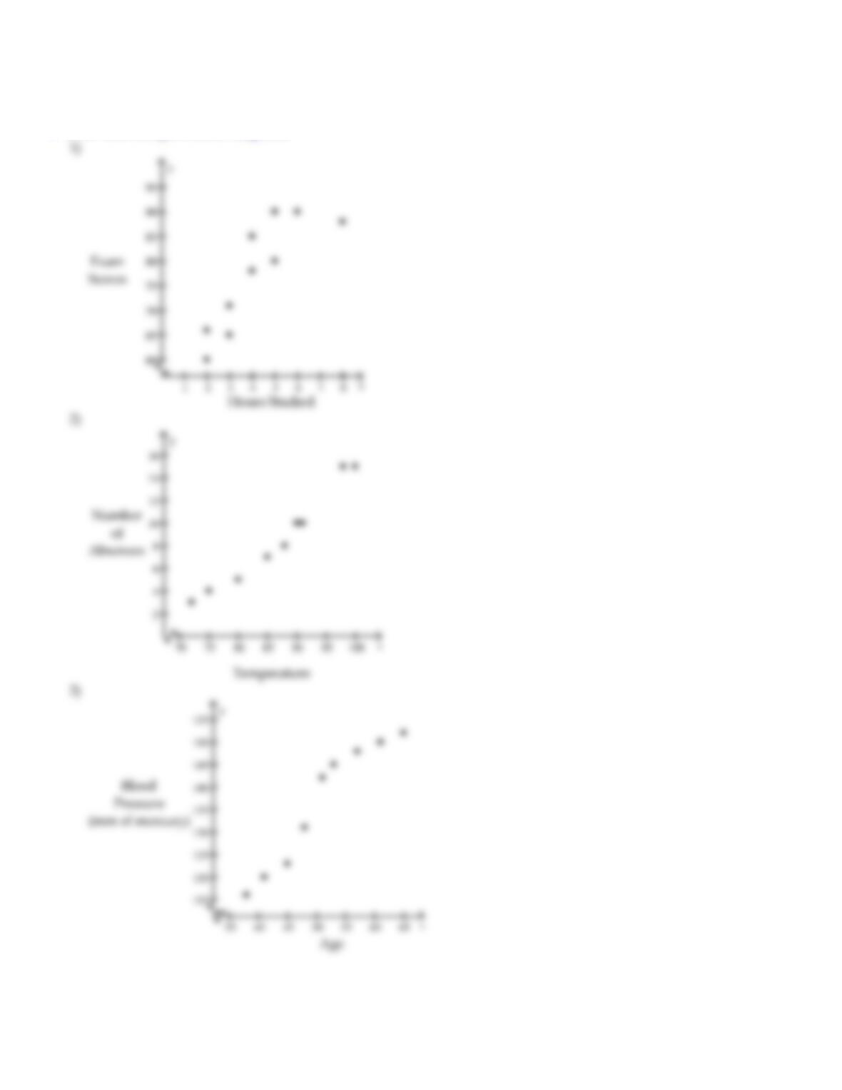
Ch.4 DescribingtheRelationbetweenTwoVariables
AnswerKey
4.1 ScatterDiagramsandCorrelation
1 Drawandinterpretscatterdiagrams.
Page134
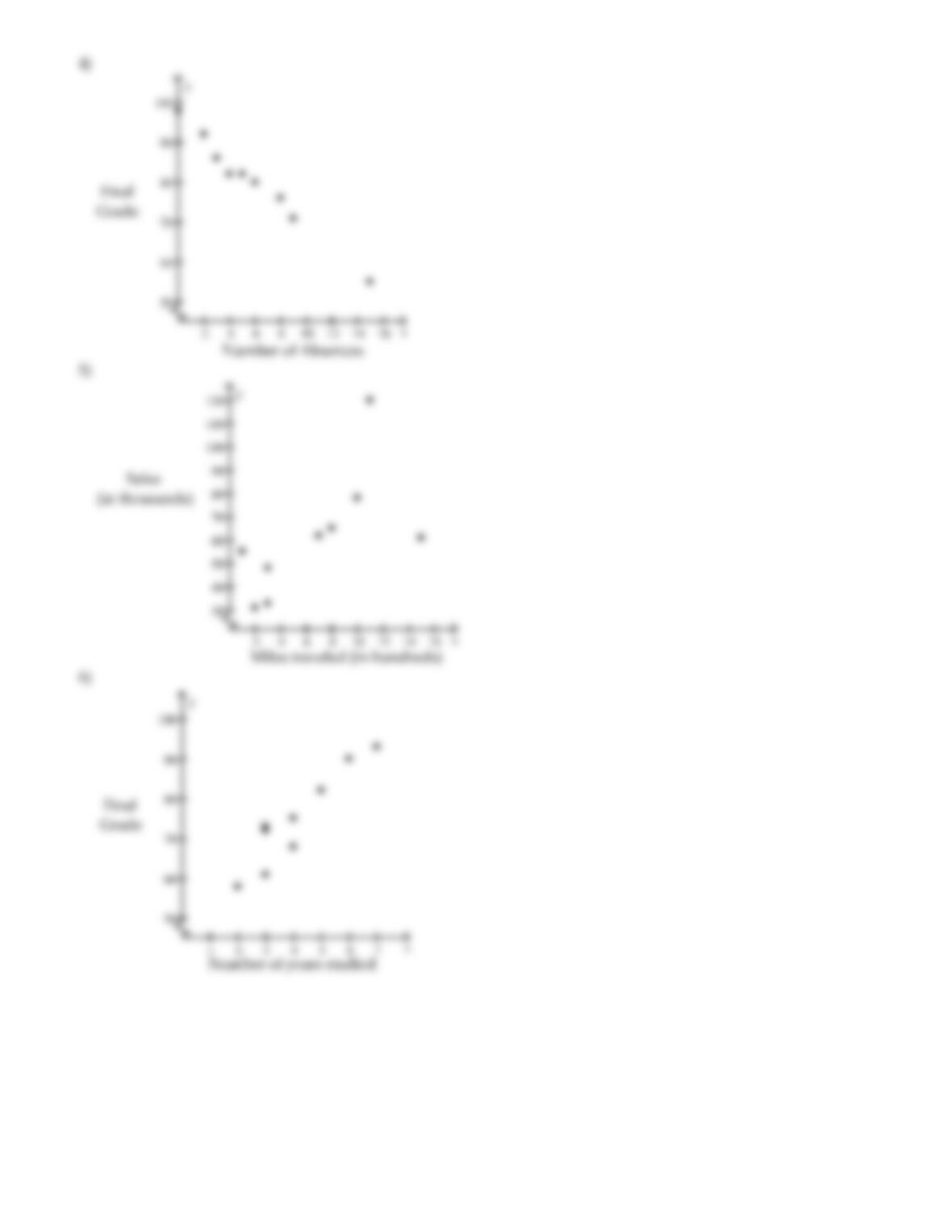
Page135
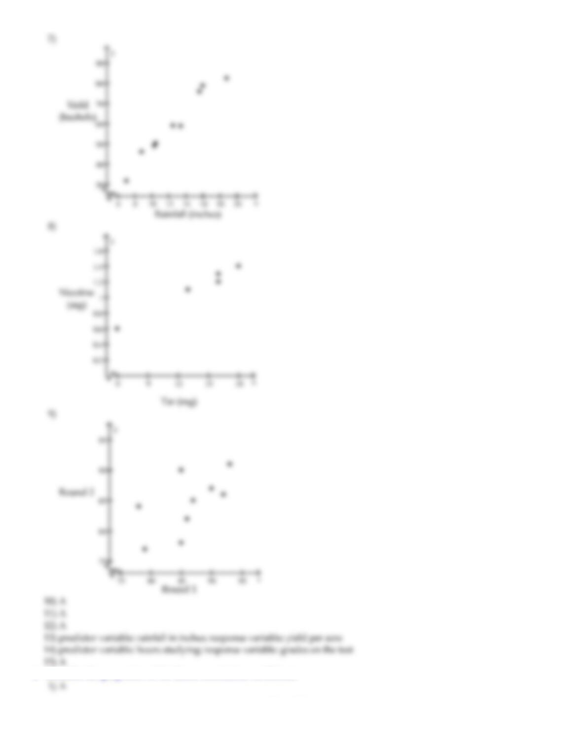
2 Describethepropertiesofthelinearcorrelationcoefficient.
Page136
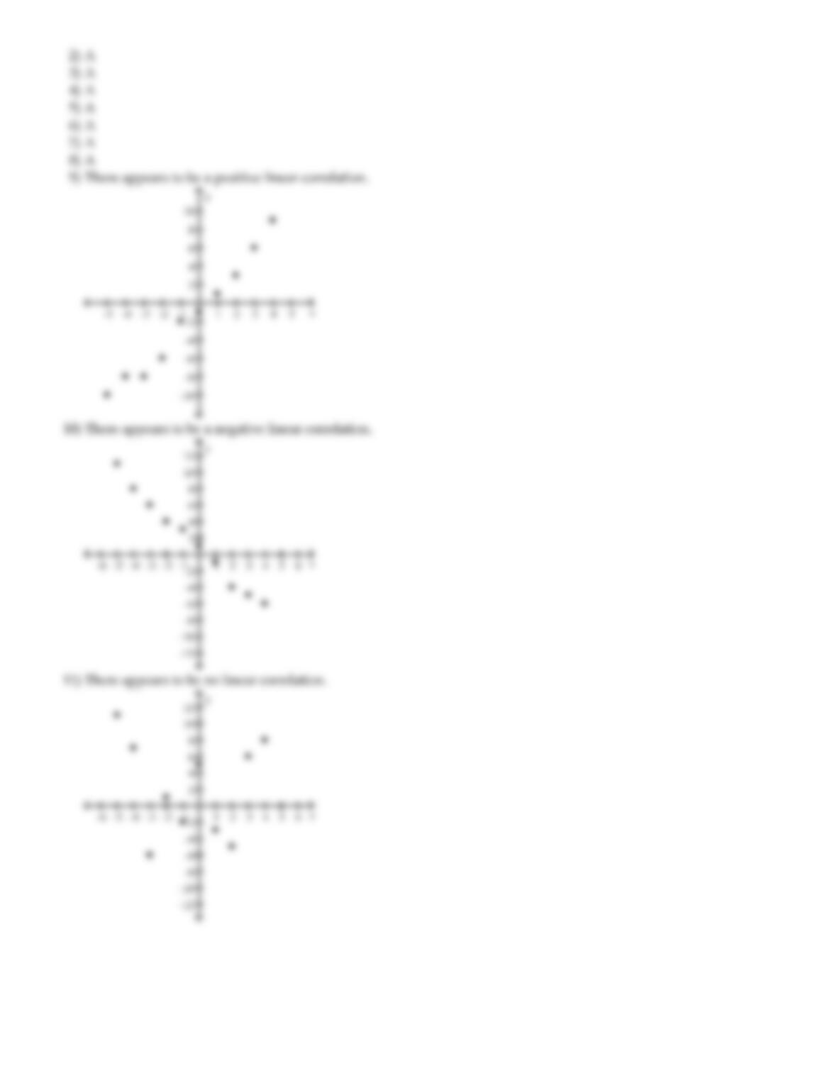
Page137
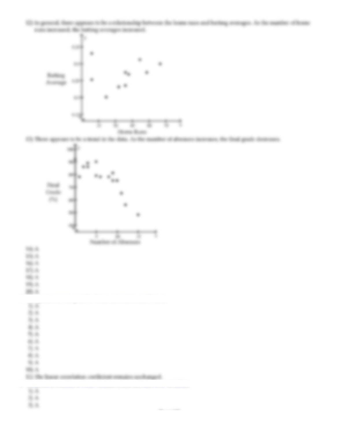
3 Computeandinterpretthelinearcorrelationcoefficient.
4 Determinewhetheralinearrelationexistsbetweentwovariables.
Page138
5 Explainthedifferencebetweencorrelationandcausation.
4.2 Least–SquaresRegression
1 Findtheleast–squaresregressionlineandusethelinetomakepredictions.
Page139
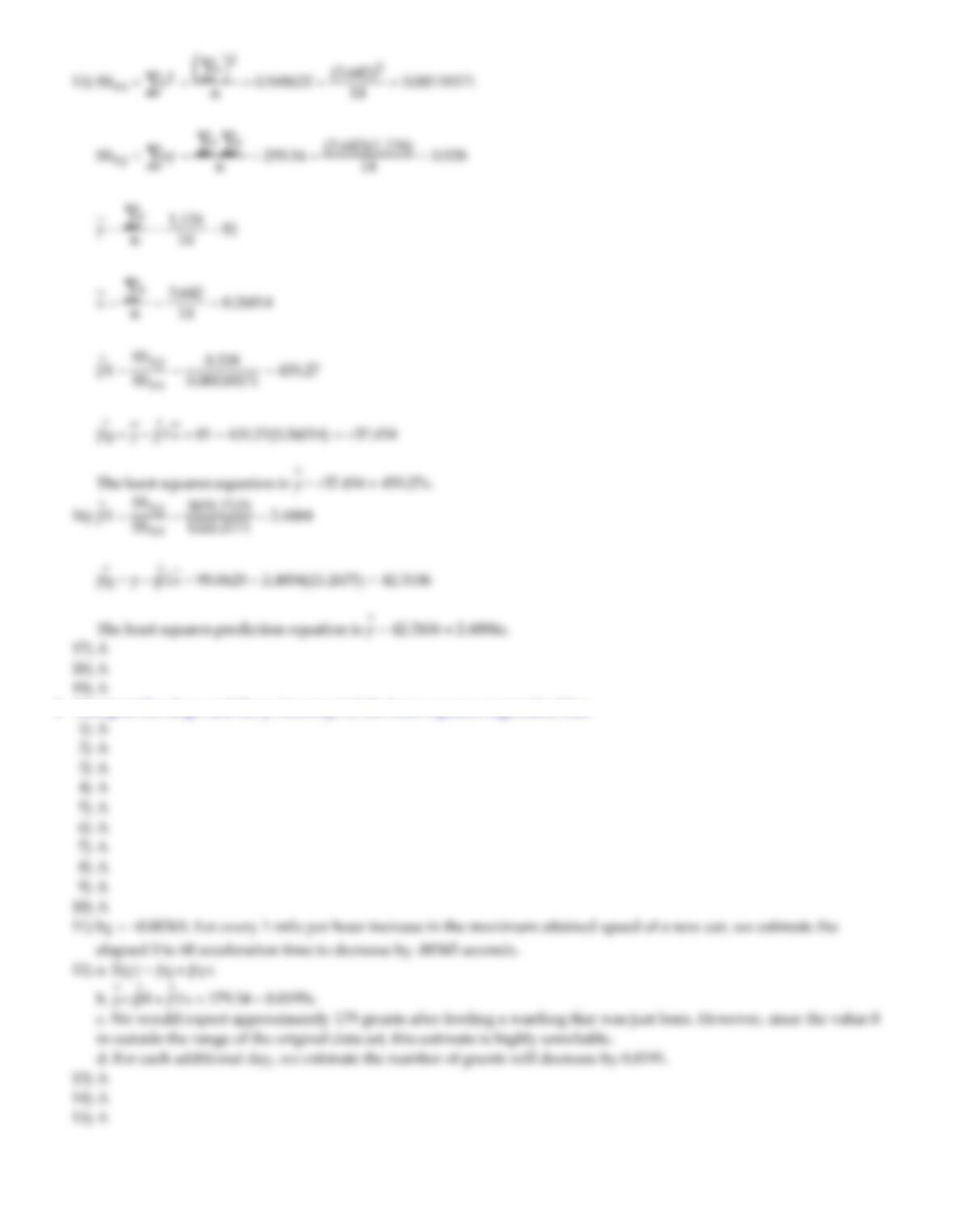
2 Interprettheslopeandthey–interceptoftheleast–squaresregressionline.
Page140
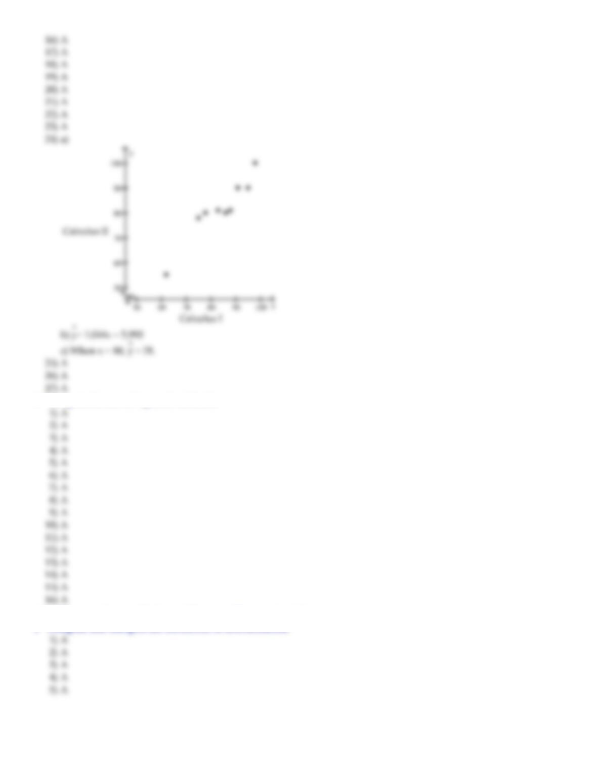
3 Computethesumofsquaredresiduals.
4.3 DiagnosticsontheLeast–SquaresRegressionLine
1 Computeandinterpretthecoefficientofdetermination.
Page141
2 Performresidualanalysisonaregressionmodel.
3 Identifyinfluentialobservations.
4.4 ContingencyTablesandAssociation
1 Computethemarginaldistributionofavariable.
2 Usetheconditionaldistributiontoidentifyassociationamongcategoricaldata.
Page142
3 ExplainSimpsonʹsParadox.
4.5 NonlinearRegression:Transformations(onCD)
1 Convertbetweenexponentialandlogarithmicexpressions.
2 Simplifylogarithmicexpressions.
Page143
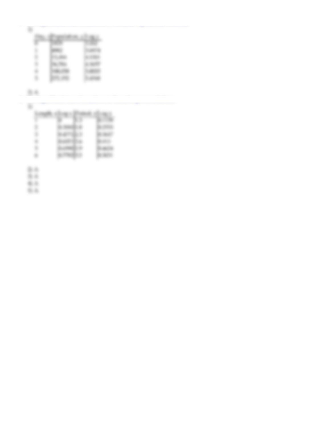
3 Uselogarithmictransformationstolinearizeexponentialrelations.
4 Uselogarithmictransformationstolinearizepowerrelations.
Page144