1) which of the following is real capital?
a.a pair of stockings
b.a construction crane
c.a savings account
d.a share of ibm stock
2) an owner’s liability for the debts of a business is:
a.limited in a corporation to the assets of preferred stockholders.
b.limited in a corporation to the assets of bondholders.
c.limited to the owner’s investment in a single proprietorship.
d.unlimited in a partnership.
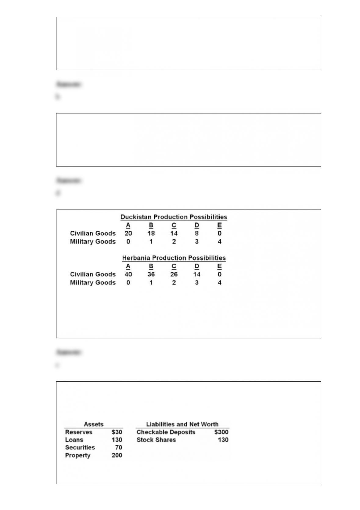
3)
refer to the above tables. opportunity costs are:
a.constant in both duckistan and herbania.
b.larger in duckistan than in herbania.
c.increasing in both duckistan and herbania.
d.increasing in duckistan and constant in herbania.
4) The following consolidated balance sheet for the commercial banking system.
Assume the required reserve ratio is 10 percent. All figures are in billions.
Refer to the above data. After the deposit of $10 billion of new currency, the maximum
amount by which this commercial banking system can expand the supply of money by
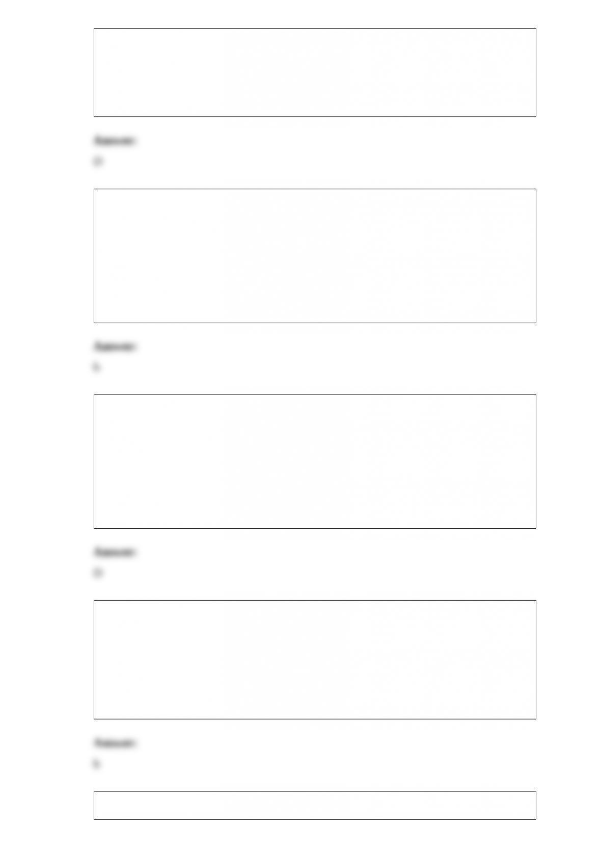
lending is:
A.$9 billion.
B.$45 billion.
C.$36 billion.
D.$90 billion.
5) protective tariffs are:
a.maximum limits on the quantity or total value of specific products imported to a
nation.
b.excise taxes or duties placed on imported products.
c.licensing requirements, unreasonable quality standards, and the like designed to
impede imports.
d.government payments to domestic producers to reduce the world prices of exported
goods.
6) Suppose the economy is operating at its full-employment-noninflationary GDP and
the MPC is 0.75. The Federal government now finds that it must increase spending on
military goods by $21 billion in response to deterioration in the international political
situation. To sustain full-employment-noninflationary GDP government must:
A.reduce taxes by $28 billion.
B.reduce transfer payments by $21 billion.
C.increase taxes by $21 billion.
D.increase taxes by $28 billion.
7) suppose you go to a doctor but your health insurance plan does not reimburse you
because you have not yet paid enough out-of-pocket for the year to qualify for
insurance benefits. this is an example of:
a.coinsurance.
b.a deductible.
c.monopsony power.
d.a deferred benefit plan.
8) refer to the above diagram. line (2) reflects the long-run supply curve for:
error! hyperlink reference not valid.error! hyperlink reference not valid.
a.a constant-cost industry.
b.a decreasing-cost industry.
c.an increasing-cost industry.
d.a technologically progressive industry.
9) the m&m experiment demonstrated that:
a.the law of diminishing marginal utility is not valid.
b.diminishing marginal utility did not apply because differently colored m&ms taste
different.
c.marginal utility diminishes less rapidly in the presence of variety.
d.marginal utility diminishes more rapidly in the presence of variety.
10) The incidence of a tax pertains to:
A.the degree to which it alters the distribution of income.
B.how easy it is to evade the tax.
C.who actually bears the burden of a tax.
D.the progressiveness or regressiveness of tax rates.
11) When aggregate demand declines, some firms may reduce employment rather than
wages because wage reductions may:
A.not be possible due to the minimum wage law.
B.increase the cost of raising money capital.
C.reduce the demands for their products.
D.may set off a price war.
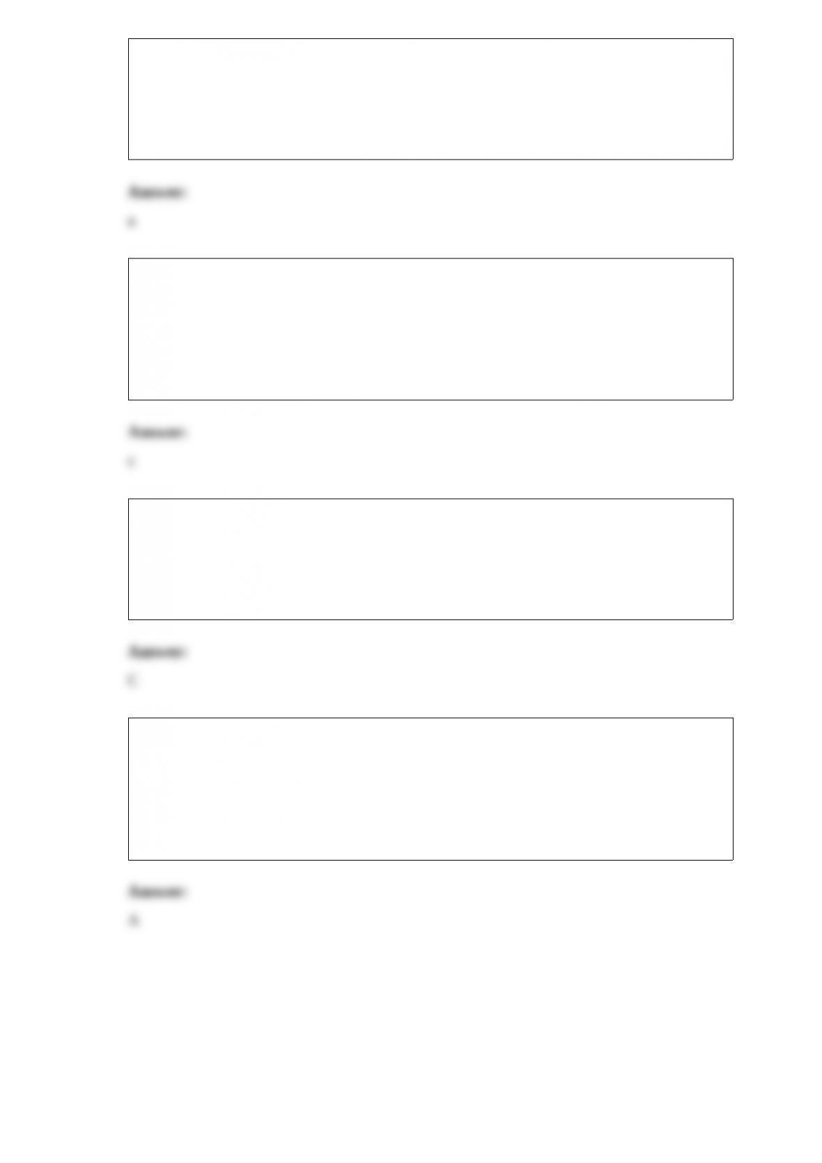
12)
Refer to the above diagrams. The solid lines are production possibilities curves; the
dashed lines are trading possibilities curves. The trading possibilities curves suggest
that the terms of trade are:
A.1.5 beers for 1 pizza.
B.1 beer for 2 pizzas.
C.2 beers for 1 pizza.
D.1 beer for 1.5 pizzas.
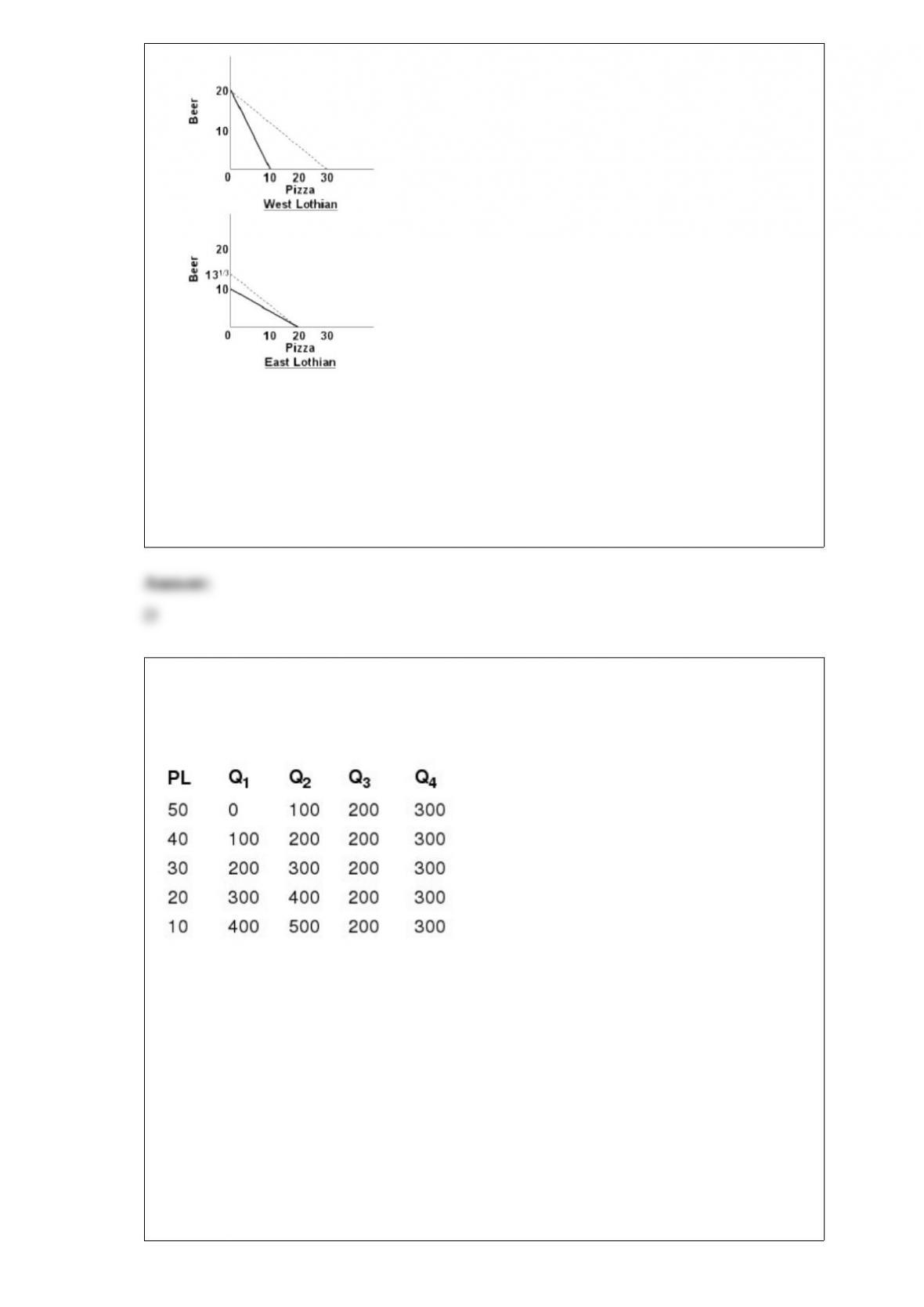
13) Below are price level (PL) and output (Q) combinations to describe aggregate
demand and aggregate supply curves: (1) PL and Q1 are AD1. (2) PL and Q2 are AD2.
(3) PL and Q3 are ASLR1. (4) PL and Q4 are ASLR2.
(a)Use the graph below to graph AD1, AD2, ASLR1, and ASLR2. Label the vertical
axis as the price level and the horizontal axis as real output (Q).
(b)If the economy is initially in equilibrium where AD1 and ASLR1 intersect, what will
the price level and real output be?
(c)If over time, the economy grows from ASLR1 to ASLR2, what will be the
equilibrium price level and real output?
(d)Assume a monetary rule is adopted that increases the money supply proportionate to
the increase in aggregate supply. Aggregate demand will increase from AD1 to AD2, so
what will the equilibrium price level and real output be?
(e)Mainstream economists would argue that velocity is unstable, so a constant increase
in the money supply might not shift AD1 all the way to AD2. It might also be the case
that the constant increase in the money supply might shift AD2 beyond its expected
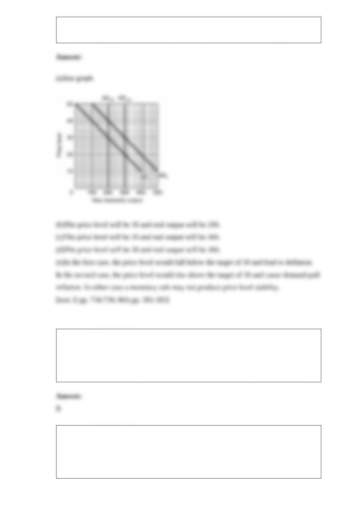
level of output. For both cases, explain what mainstream economists think will happen
to the price level.
14) The equilibrium interest rate equates:
A.nominal and real interest rates.
B.the quantities demanded and supplied of loanable funds.
C.consumption and saving.
D.taxes and government spending.
15) supporters of offshoring claim that its benefits include:
a.increased demand for workers in complementary jobs.
b.keeping u.s. firms profitable by lowering production costs.
c.reduced prices for consumers.
d.all of these.
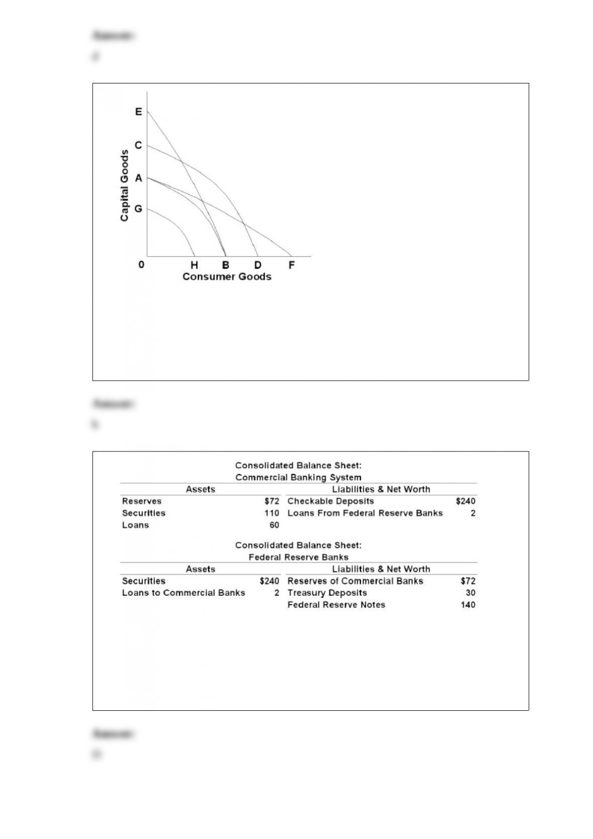
16)
refer to the above diagram. which one of the following would shift the production
possibilities curve from pp1 to pp2?
a.worsening of the aids epidemic
b.immigration of skilled workers into the economy
c.an increase in consumer prices
d.a reduction in hourly wages
17)
Which of the following is correct? When the Federal Reserve buys government
securities from the public, the money supply:
A.contracts and commercial bank reserves increase.
B.expands and commercial bank reserves decrease.
C.contracts and commercial bank reserves decrease.
D.expands and commercial bank reserves increase.