Chapter 9—Correlation
MULTIPLE CHOICE QUESTIONS
9.1 + In plotting the relationship between the incidence of breast cancer and the level of
vitamin D in the body, we would most likely plot
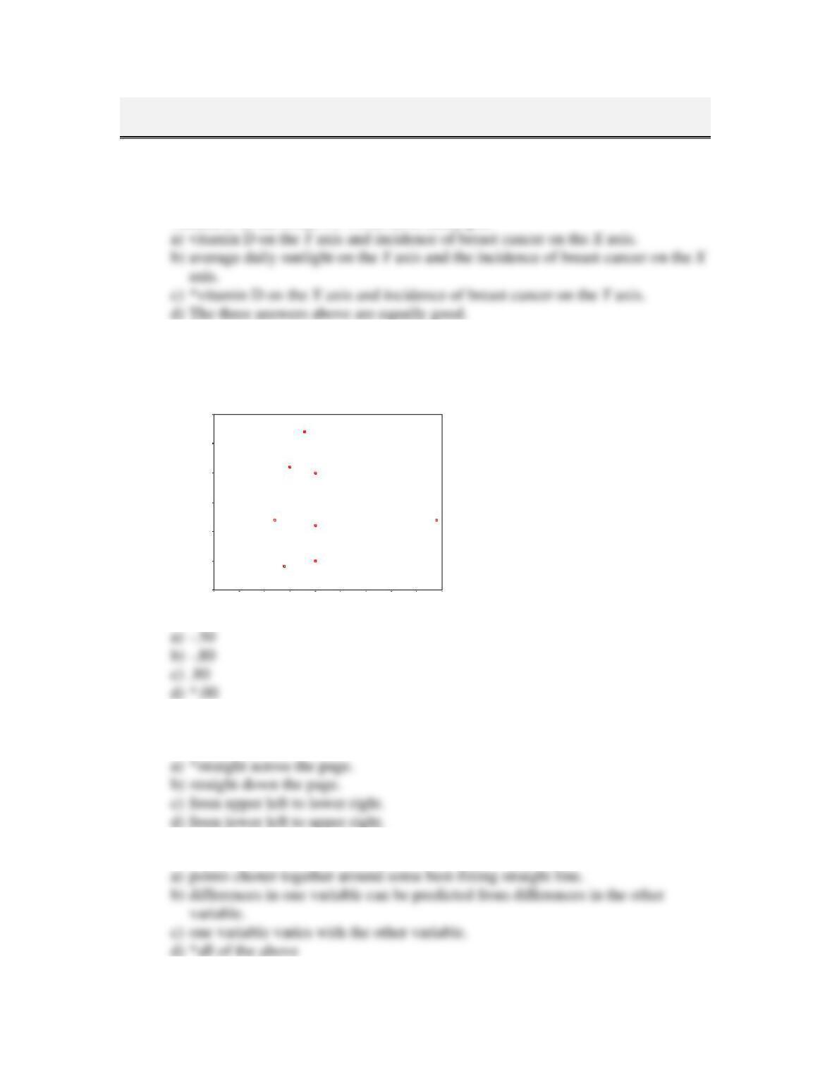
9.2 The following is a scatterplot of data that my students collected concerning the
relationship between the cost of chocolate chip cookies and their rated quality.
The correlation between the two variables is most likely to be
Price
5.55.04.54.03.53.02.52.01.51.0
Rating
4.5
4.0
3.5
3.0
2.5
2.0
1.5
9.3 In the previous question, a “best–fitting” line drawn through the data points would
most likely go
9.4 The correlation between two variables is a measure of the degree to which
Test Bank
270
9.5 + Early in the correlation chapter the author showed figures in which he drew
vertical and horizontal lines at the mean of each variable to cut the graph into four
quadrants. When there is a high positive correlation between two variables, we
would expect most of the data points to fall
9.6 + The correlation between two variables is defined as
9.7 Spearman’s correlation coefficient (rS ) applies to
9.8 When we restrict the range of X or Y, we may
9.9 When we use heterogeneous subsamples of data, such as older and younger
subjects, the resulting correlation between intelligence and education could
9.10 When we say that the correlation between Age and test Performance is
significant, we mean
Chapter 9
271
9.11 + If the correlation between the rating of cookie quality and cookie price is .30, and
the critical value from the table of significance of correlation coefficients is .35,
we would say that
9.12 A dichotomous variable is one that
9.13 The difference between a point biserial coefficient and a normal Pearson
correlation coefficient is that
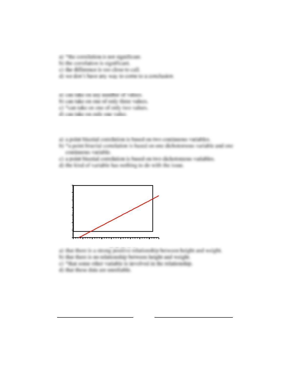
9.14 The data illustrated in the graph below suggest
1 3 0
1 4 0
1 5 0
1 6 0
1 7 0
1 8 0
1 9 0
2 0 0
55575961636567697173
W e ig h t
9.15 + Inglehart (1990) presented data on the relationship between income (as
represented by a country’s Gross National Product), and reported Satisfaction
With Life for 24 countries. These data speak to the issue of whether people in
countries with a higher standard of living also report greater satisfaction. The data
have been sorted by Satisfaction.
Country
Satisf
GNP
Country
Satisf
GNP
Portugal
5.5
1,900
Canada
7.2
13,300
Greece
5.8
3,800
Belgium
7.3
9,100
Japan
6.4
10,700
Britain
7.5
9,000
Test Bank
Spain
6.5
4,200
U.S.A.
7.55
15,700
Italy
6.5
6,300
Ireland
7.7
5,000
South Africa
6.6
2,100
Luxemburg
7.75
9,400
France
6.6
9,900
Finland
7.75
10,700
Argentina
6.72
2,200
Norway
7.85
14,000
Hungary
6.95
4,300
Australia
7.9
10,100
Austria
7.1
9,300
Switzerland
7.95
15,900
Netherlands
7.2
9,300
Denmark
8.0
11,000
W. Germany
7.2
11,000
Sweden
8.0
11,900
Visual inspection of these data would suggest that the correlation is closest to
9.16 In the scatterplot for the data in the previous question, the biggest outliers are
likely to be
9.17 + A reliable correlation is one that
9.18 + Which of the following represents a closer relationship between two variables?
9.19 The example showing a negative relationship between speed and accuracy tells us
that
9.20 A curvilinear relationship is one in which
Chapter 9
273
9.21 We can often use a Pearson correlation even when a relationship is curvilinear.
This is because
9.22 The covariance will always
9.23 + For a given set of data the covariance between X and Y is .80. The standard
deviation of X is 2.0, and the standard deviation of Y is 3.0. The resulting
correlation is closest to
9.24 + If high scores on X are paired with low scores on Y, the covariance is going to be
9.25 Which of the following is the formula for the covariance?
9.26 + For the following data, XY is equal to
X 2 4 5
Y 2 3 4
Test Bank
9.27 If the correlation between two variables is .76, and the sample size is large, we
can conclude that
9.28 + When the data are in the form of ranks we
9.29 When we have a relationship that is continually rising, but the line showing the
relationship is not necessarily straight, we call this a _______ relationship.
9.30 + If we look at the correlation between college admissions test scores and
subsequent performance in college for all admitted applicants, we are likely to
9.31 + Which of the following is NOT a reason to explain why infant mortality increased
with the number of physicians?
9.32 When we say that a correlation coefficient is statistically significant, we mean that
Chapter 9
9.33 The correlation in the population is denoted by
9.34 In testing the significance of a correlation coefficient, the degrees of freedom are
9.35 An intercorrelation matrix is one that
9.36 If one of our variables is a dichotomy, the correlation we compute is
9.38 + A newspaper headline writer found that the more adjectives she put in the titles of
her articles, the greater the number of newspapers that were sold that day. This
relationship between numbers of adjectives and newspaper sales must be
9.39 The covariance between height and running speed on the State College track team
was equal to –28.21. This tells us that the
Test Bank
9.40 A _______ refers to the degree of the relationship between two or more variables.
9.41 Which r-value represents the strongest correlation?
9.42 The correlation between amount of caffeine consumed and nervous behavior was
found to be .30. What conclusion can be drawn from this finding?
9.43 The covariance measure is
9.44 If the R squared between brain size and IQ is .09 then
9.45 Which of the following is the most accurate statement?
Chapter 9
277
9.46 Professor Falls wants to determine if there is a relationship between frequent
hearing of a startle stimulus and hearing loss. He ran a regression and obtained an
r value of .60. Which of the following best summarizes what this result means?
9.47 A correlation was computed between amount of exercise people do and people’s
overall happiness. A significant correlation was found, such that the more people
exercise, the happier they are. What is the best conclusion to draw from this
finding?
9.48 We want to demonstrate that a relationship exists between optimism and
happiness. We are not concerned with trying to demonstrate that one variable
causes the other. What type of statistical test can be use to see if a relationship
exists between the variables?
9.49 Which of the following pairs is most likely to be negatively correlated?
9.50 A significant correlation is one which
9.51 We look at a number of states and record the number of auto fatalities last year
and the state’s maximum speed limit, trying to show that high speed limits are
dangerous. This is an example of
Test Bank
278
True/False Questions
dichotomous variables.
increase, so does foot size.
studying. The criterion variable is exam scores.
who are highly depressed are reasonably likely to be highly anxious.
variables.
groups.
dichotomous.
Chapter 9
279
OPEN-ENDED QUESTIONS
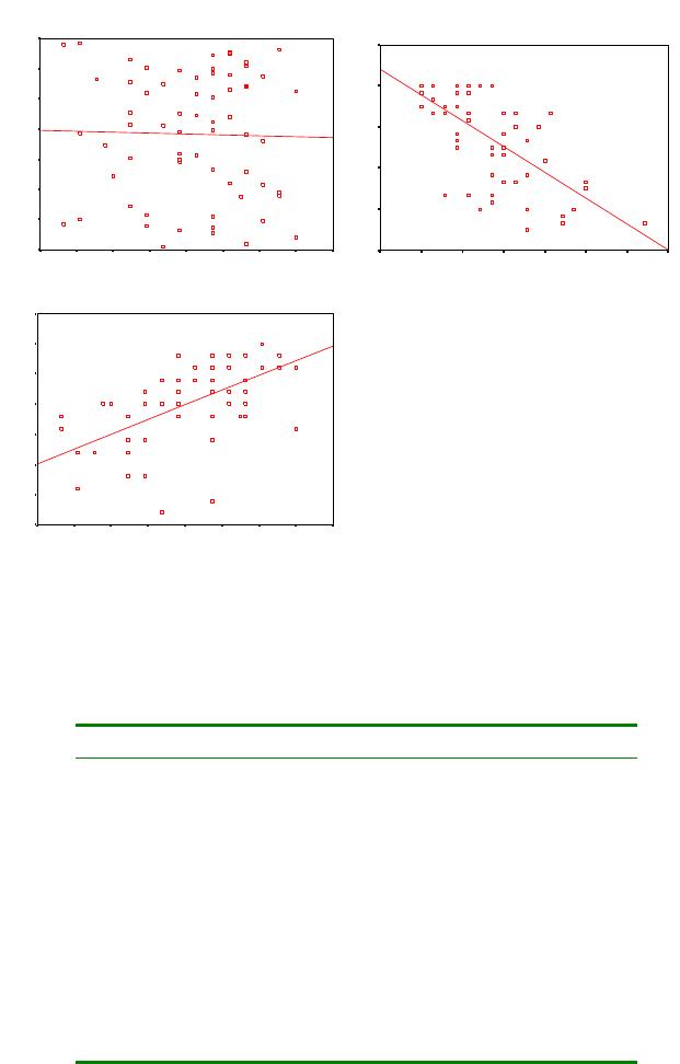
9.62 Indicate the types of relationships illustrated in the following graphs. (e.g.,
positive, negative, no relationship, curvilinear).
a.
4.24.03.83.63.43.23.02.82.6
140
120
100
80
60
40
20
0
b.
4.03.53.02.52.01.51.0.5
4.5
4.0
3.5
3.0
2.5
2.0
c.
4.24.03.83.63.43.23.02.82.6
5.5
5.0
4.5
4.0
3.5
3.0
2.5
2.0
9.63 Given the following pairs of data for mothers’ and fathers’ ratings of their child’s
behavior problems, what type of correlation would you expect? Explain your
answer.
Child Behavior Problem Score
Mother’s Rating
Father’s Rating
Family 1
60
70
Family 2
55
50
Family 3
30
30
Family 4
45
40
Family 5
95
100
Family 6
75
75
Family 7
50
55
Family 8
100
90
Family 9
25
30
Test Bank
280
9.64 Write a brief paragraph to summarize the data displayed in the following table.
1
2
3
4
1. Wives’ marital aggression
–
-.25*
.45**
-.35*
2. Wives’ marital satisfaction
–
-.30*
.63***
3. Husbands’ marital aggression
–
-.30*
4. Husbands’ marital satisfaction
–
N = 100; * p < .05; ** p < .01; *** p < .001
9.65 Make a scatterplot of the following data and draw a line of best fit.
Self-esteem
Grades
10.00
83.00
9.00
97.00
8.00
92.00
7.00
83.00
7.00
93.00
6.00
97.00
6.00
75.00
6.00
68.00
5.00
59.00
4.00
65.00
9.66 Calculate the correlation coefficient for the previous data. Is it significant? Write
a brief statement to explain the results.
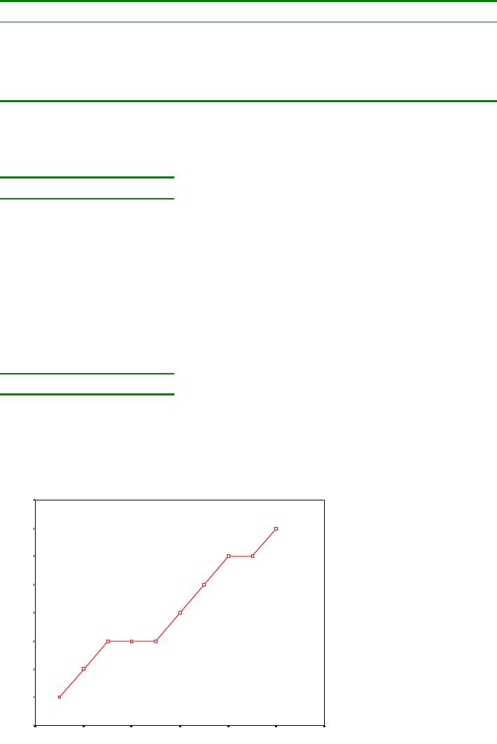
9.67 Describe the following graph.
121086420
8
7
6
5
4
3
2
1
0
9.68 Give an example of a relationship that may be effected by the heterogeneity of a
sample. Explain your example clearly.
Chapter 9
281
9.69 Give an example of a relationship that is effected by restricted range. Explain
your example clearly.
9.70 Calculate and interpret the correlation between the following variables.
X
Y
5.00
2.00
5.00
1.00
5.00
2.00
4.00
2.00
4.00
3.00
3.00
4.00
3.00
4.00
2.00
3.00
2.00
2.00
9.71 Give an example of a:
a) positive relationship
b) negative relationship
c) curvilinear relationship
Answers to Open-ended Questions
Chapter 9.
Test Bank
282