Name:
Class:
Date:
chapter 8
Indicate whether the statement is true or false.
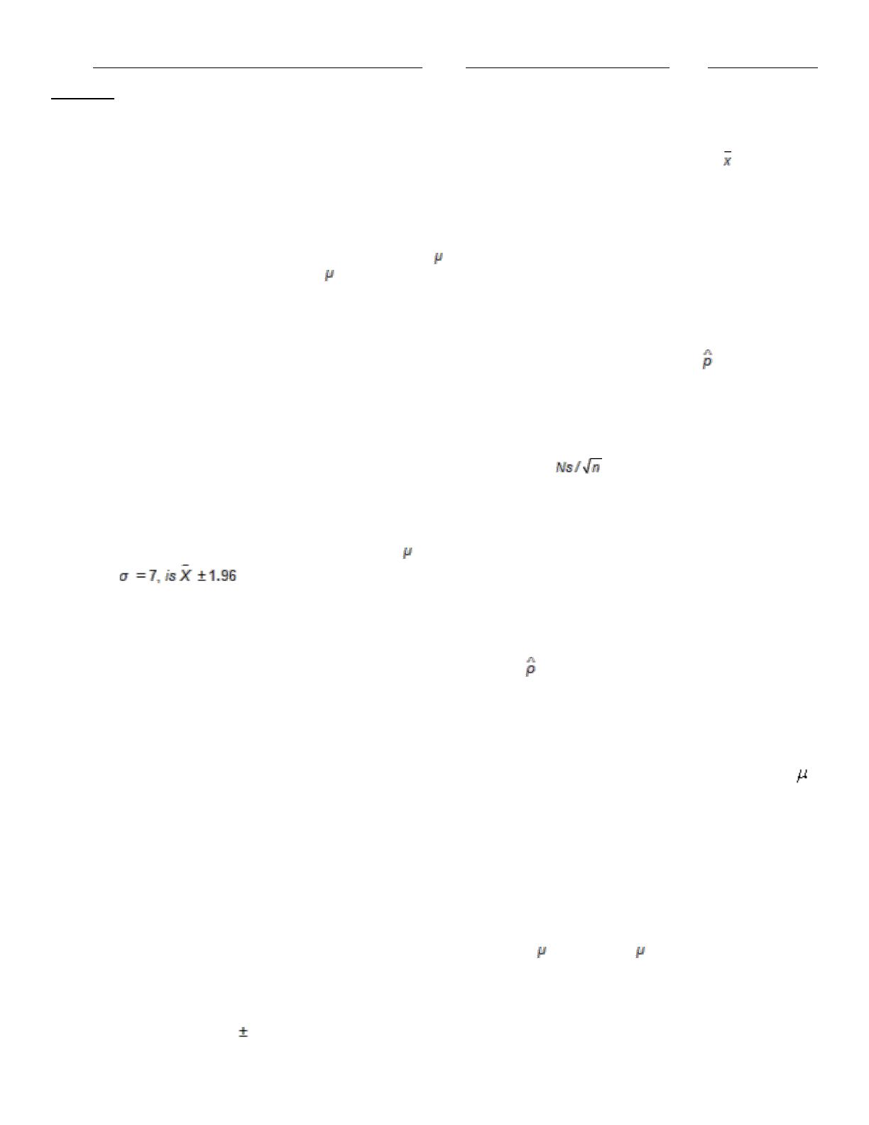
1. When samples of size n are drawn from a population, then the sampling distribution of the sample mean is
approximately normal, provided that n is reasonably large.
a.
True
b.
False
2. A 90% confidence interval estimate for a population mean is determined to be 72.8 to 79.6. If the confidence level is
reduced to 80%, the confidence interval for becomes narrower.
a.
True
b.
False
3. The lower limit of the 95% confidence interval for the population proportion p, given that n = 300; and = 0.10 is
0.1339.
a.
True
b.
False
4. The approximate standard error of the point estimate of the population total is .
a.
True
b.
False
5. The 95% confidence interval for the population mean , given that the sample size n = 49 and the population standard
deviation
a.
True
b.
False
6. If the standard error of the sampling distribution of the sample proportion is 0.0324 for samples of size 200, then the
population proportion must be 0.30.
a.
True
b.
False
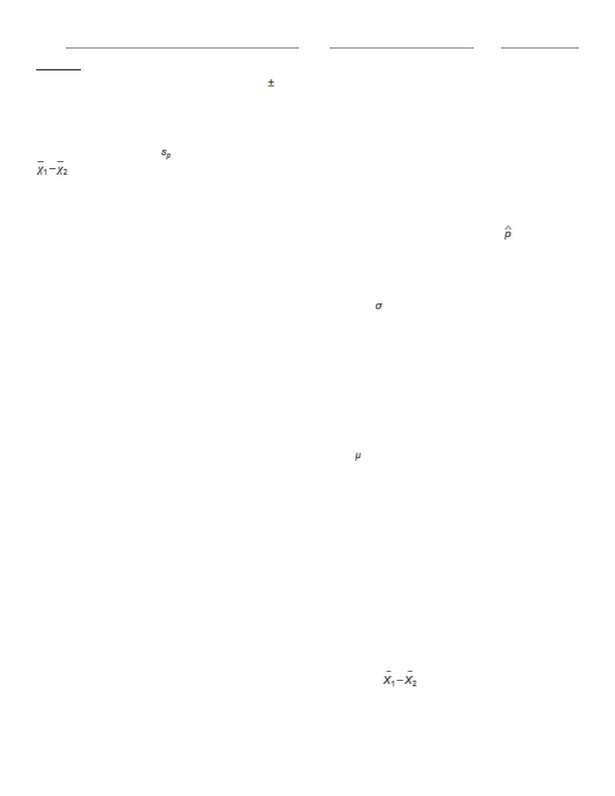
7. We can form a confidence interval for the population total T by finding a confidence interval for the population mean
in the usual way, and then multiplying the lower and upper limits the confidence interval by the population size N.
a.
True
b.
False
8. Samples of exam scores for employees before and after a training class would be examples of paired data
a.
True
b.
False
9. In order to construct a confidence interval estimate of the population mean , the value of must be given.
a.
True
b.
False
10. The interval estimate 18.5 2.5 was developed for a population mean when the sample standard deviation s was 7.5.
Name:
Class:
Date:
chapter 8
Had s equaled 15, the interval estimate would be 37 5.0.
a.
True
b.
False
11. In developing confidence interval for the difference between two population means using two independent samples,
we use the pooled estimate in estimating the standard error of the sampling distribution of the sample mean difference
if the populations are normal with equal variances.
a.
True
b.
False
12. The upper limit of the 90% confidence interval for the population proportion p, given that n = 100; and = 0.20 is
0.2658.
a.
True
b.
False
13. In developing a confidence interval for the population standard deviation , we make use of the fact that the sampling
distribution of the sample standard deviation s is not the normal distribution or the t-distribution, but rather a right-skewed
distribution called the chi-square distribution, which (for this procedure) has n – 1 degrees of freedom.
a.
True
b.
False
14. The t-distribution and the standard normal distribution are practically indistinguishable as the degrees of freedom
increase.
a.
True
b.
False
15. If a sample has 20 observations and a 95% confidence estimate for is needed, the appropriate value of t–multiple is
2.093
a.
True
b.
False
16. A confidence interval is an interval estimate for which there is a specified degree of certainty that the actual true value
of the population parameter will fall within the interval.
a.
True
b.
False
17. In general, increasing the confidence level will narrow the confidence interval, and decreasing the confidence level
widens the interval.
a.
True
b.
False
18. If two random samples of sizes 30 and 35 are selected independently from two populations whose means are 85 and
90, then the mean of the sampling distribution of the sample mean difference, , equals 5.
a.
True
b.
False
Name:
Class:
Date:
chapter 8
19. In determining the sample size n for estimating the population proportion p, a conservative value of n can be obtained
by using 0.50 as an estimate of p.
a.
True
b.
False
20. If we cannot make the strong assumption that the variances of two samples are equal, then we must use the pooled
standard deviation in calculating the standard error of a difference between the means.
a.
True
b.
False
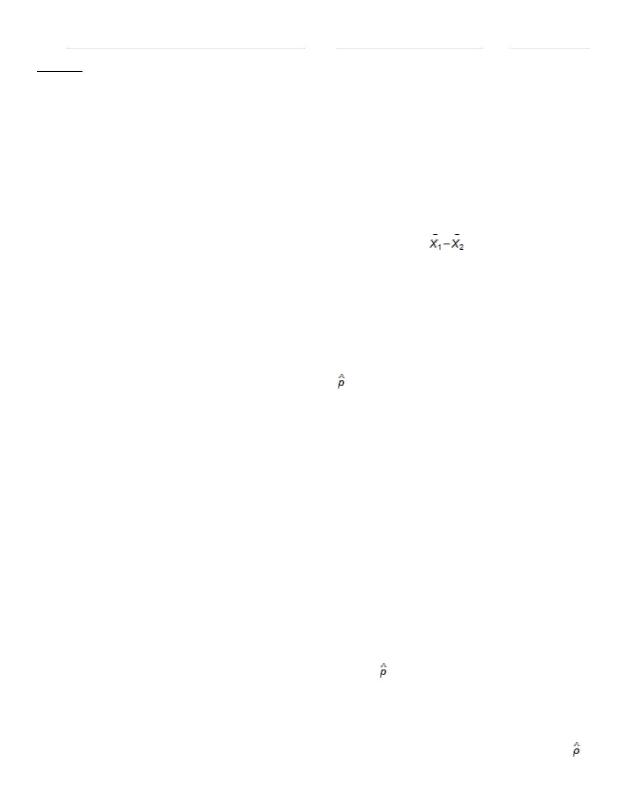
21. If two random samples of size 40 each are selected independently from two populations whose variances are 35 and
45, then the standard error of the sampling distribution of the sample mean difference, , equals 1.4142.
a.
True
b.
False
22. The confidence interval for the population standard deviation s is centered at the point estimate, the sample standard
deviation s.
a.
True
b.
False
23. The mean of the sampling distribution of the sample proportion , when the sample size n = 100 and the population
proportion p = 0.15, is 15.0.
a.
True
b.
False
24. The degrees of freedom for the t and chi-square distributions is a numerical parameter of the distribution that defines
the precise shape of the distribution.
a.
True
b.
False
25. In general, the paired-sample procedure is appropriate when the samples are naturally paired in some way and there
is a reasonably large positive correlation between the pairs. In this case, the paired-sample procedure makes more
efficient use of the data and generally results in narrower confidence intervals.
a.
True
b.
False
26. If two samples contain the same number of observations, then the data must be paired.
a.
True
b.
False
27. The standard error of the sampling distribution of the sample proportion , when the sample size n = 50 and the
population proportion p = 0.25, is 0.00375.
a.
True
b.
False
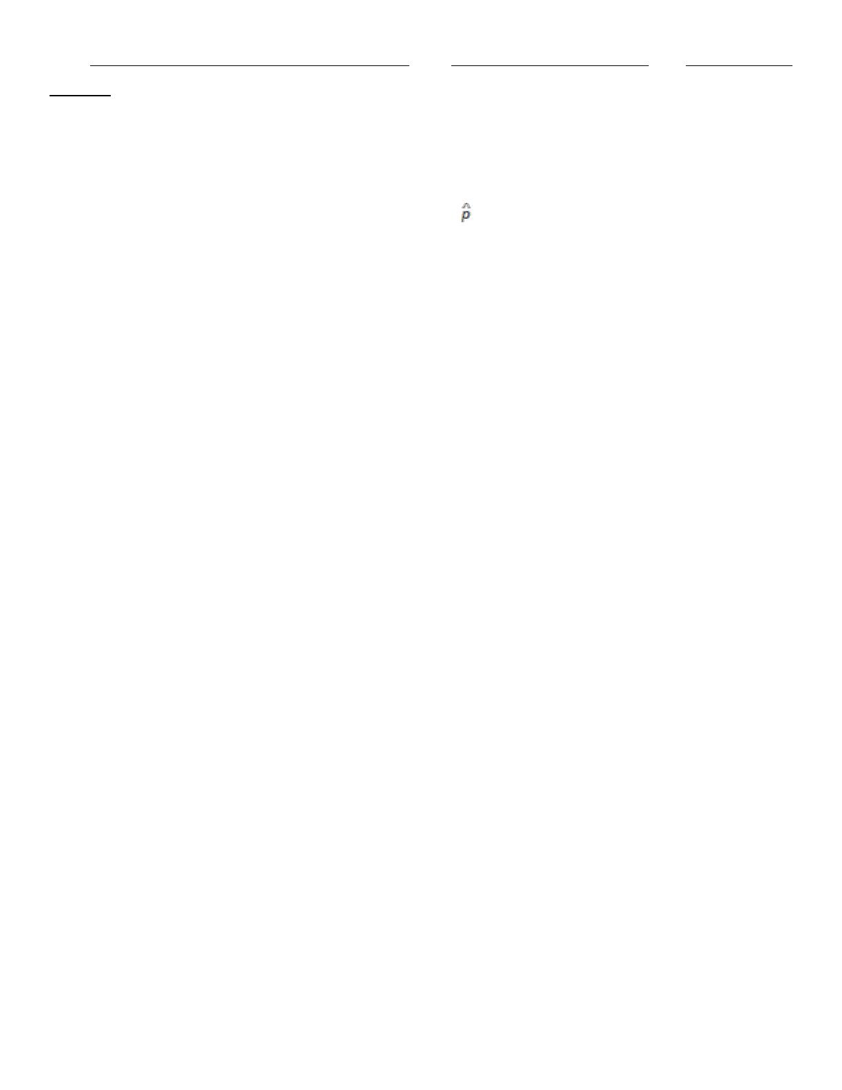
28. As a general rule, the normal distribution is used to approximate the sampling distribution of the sample proportion
Name:
Class:
Date:
chapter 8
only if the sample size n is greater than 30.
a.
True
b.
False
29. If a random sample of size 250 is taken from a population, where it is known that the population proportion p = 0.4,
then the mean of the sampling distribution of the sample proportion is 0.60.
a.
True
b.
False
Indicate the answer choice that best completes the statement or answers the question.
30. After calculating the sample size needed to estimate a population proportion to within 0.05, you have been told that
the maximum allowable error (B) must be reduced to just 0.025. If the original calculation led to a sample size of 1000, the
sample size will now have to be:
a.
2000
b.
4000
c.
1000
d.
8000
31. If you are constructing a confidence interval for a single mean, the confidence interval will with a decrease in the
sample size.
a.
decrease
b.
increase
c.
stay the same
d.
increase or decrease, depending on the sample data
32. If you decrease the confidence level, the confidence interval .
a.
decreases
b.
increases
c.
stays the same
d.
may increase or decrease, depending on the sample data
33. Two independent samples of sizes 20 and 25 are randomly selected from two normal populations with equal
variances. In order to test the difference between the population means, the test statistic is:
a.
a standard normal random variable
b.
approximately standard normal random variable
c.
t-distributed with 45 degrees of freedom
d.
t-distributed with 43 degrees of freedom
34. Suppose there are 500 accounts in a population. You sample 50 of them and find a sample mean of $500. What
would be your estimate for the population total?
a.
$5,000
b.
$50,000
c.
$250,000
d.
$500,000
e.
None of these choices
35. The number of degrees of freedom needed to construct 90% confidence interval for the difference between means
Name:
Class:
Date:
chapter 8
when the data are gathered from paired samples, with 15 observations in each sample, is:
a.
30
b.
15
c.
28
d.
14
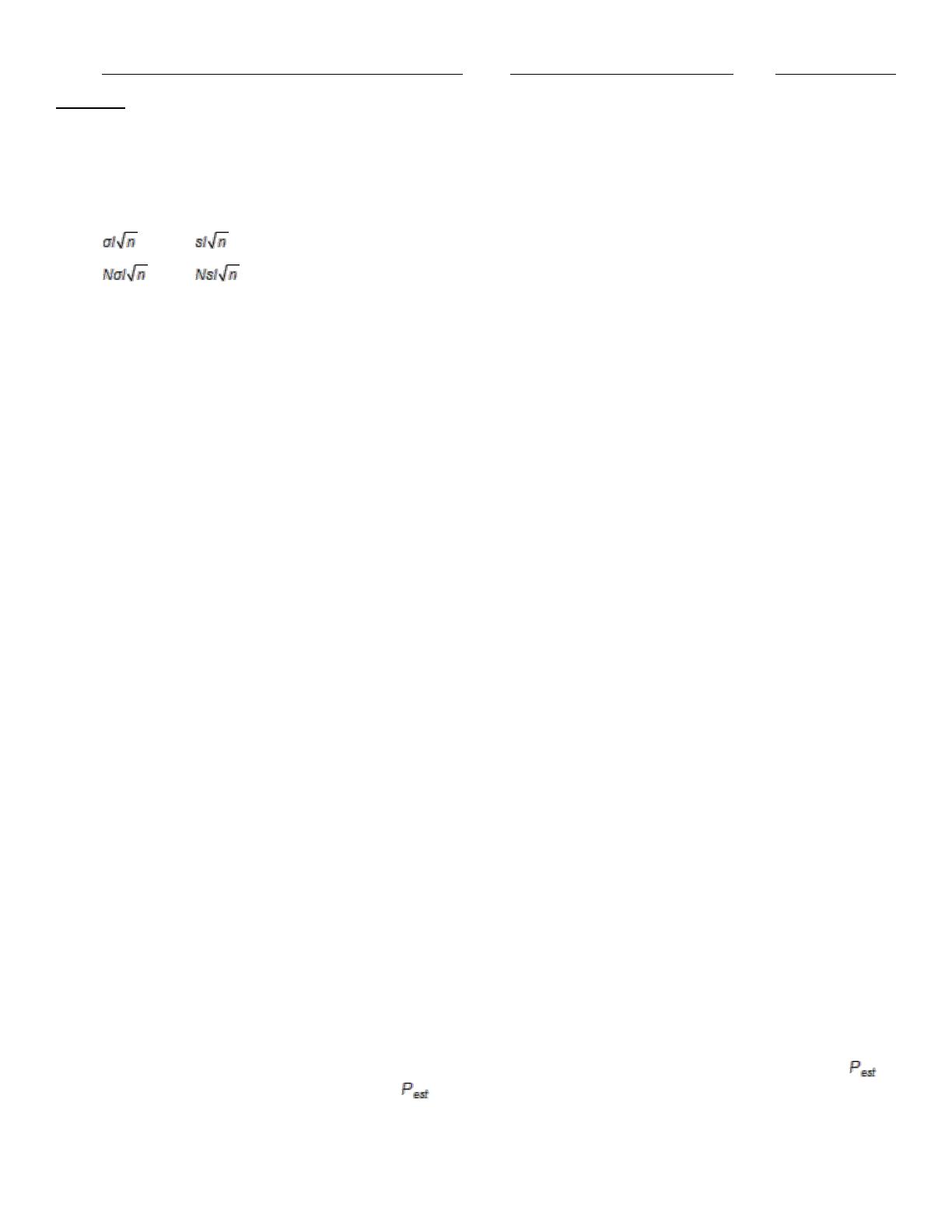
36. The approximate standard error of the point estimate of the population total is:
a.
b.
c.
d.
37. The chi-square distribution for developing a confidence interval for a standard deviation has degrees of freedom.
a.
n + 2
b.
n +1
c.
n
d.
n – 1
e.
n – 2
38. An example of a problem where the sample data would be paired is:
a.
Difference between the means of appraised and sales house prices
b.
Difference between the proportion of defective items from two suppliers
c.
Difference in the mean life of two major brands of batteries
d.
Difference in the mean salaries for graduates in two different academic fields at a university
e.
None of these options
39. From a sample of 500 items, 30 were found to be defective. The point estimate of the population proportion defective
will be:
a.
0.06
b.
30.0
c.
16.667
d.
None of the above
40. If you are constructing a confidence interval for a single mean, the confidence interval will with an increase in the
sample size.
a.
decrease
b.
increase
c.
stay the same
d.
increase or decrease, depending on the sample data
41. As the sample size increases, the t-distribution becomes more similar to the ________ distribution.
a.
normal
b.
exponential
c.
multinominal
d.
chi-square
e.
binomial
42. When you calculate the sample size for a proportion, you use an estimate for the population proportion; namely . A
conservative value for n can be obtained by using =
a.
0.01
b.
0.05

Name:
Class:
Date:
chapter 8
c.
0.10
d.
0.50
e.
1.00
43. If you increase the confidence level, the confidence interval:
a.
decreases
b.
increases
c.
stays the same
d.
may increase or decrease, depending on the sample data
44. The general form of a confidence interval is:
a.
Point Estimate = Multiple × Standard Error
b.
Point Estimate = Multiple +Standard Error
c.
Point Estimate ± Multiple × Standard Error
d.
Point Estimate = Multiple ± Standard Error
45. Two independent samples of sizes 50 and 50 are randomly selected from two populations to test the difference
between the population means, . The sampling distribution of the sample mean difference is:
a.
normally distributed
b.
approximately normal
c.
t – distributed with 98 degrees of freedom
d.
chi-squared distributed with 99 degrees of freedom
46. There are, generally speaking, two types of statistical inference. They are:
a.
sample estimation and population estimation
b.
confidence interval estimation and hypothesis testing
c.
interval estimation for a mean and point estimation for a proportion
d.
independent sample estimation and dependent sample estimation
e.
None of these choices
47. When the samples we want to compare are paired in some natural way, such as pretest/posttest for each person or
husband/wife pairs, a more appropriate form of analysis is to not compare two separate variables, but their .
a.
difference
b.
sum
c.
ratio
d.
total
e.
product
48. Confidence intervals are a function of which of the following three things?
a.
The population, the sample, and the standard deviation
b.
The sample, the variable of interest, and the degrees of freedom
c.
The data in the sample, the confidence level, and the sample size
d.
The sampling distribution, the confidence level, and the degrees of freedom
e.
The mean, median, and mode
Name:
Class:
Date:
chapter 8
49. The t-distribution for developing a confidence interval for a mean has degrees of freedom.
a.
n + 2
b.
n +1
c.
n
d.
n – 1
e.
n – 2
50. A parameter such as is sometimes referred to as a ________ parameter, because many times we need its value
even though it is not the parameter of primary interest.
a.
special
b.
random
c.
nuisance
d.
independent
e.
dependent
51. When we replace with the sample standard deviation (s), we introduce a new source of variability and the sampling
distribution becomes the:
a.
t -distribution
b.
F- distribution
c.
chi-square distribution
d.
normal distribution
52. For a given confidence level, the procedure for controlling interval length usually begins with the specification of
a.
the point estimate
b.
the population standard deviation, s
c.
the sample standard deviation, s
d.
the interval half-length, B
53. The shape of a chi-square distribution
a.
is symmetric
b.
is skewed to the left
c.
is skewed to the right
d.
depends on the sample data
54. The chi-square and F-distributions are used primarily to make inferences about population ___________.
a.
means
b.
variances
c.
medians
d.
modes
e.
proportions
A company employs two shifts of workers. Each shift produces a type of gasket where the thickness is the critical
dimension. The average thickness and the standard deviation of thickness for shift 1, based on a random sample of 40
gaskets, are 10.85 mm and 0.16 mm, respectively. The similar figures for shift 2, based on a random sample of 30
gaskets, are 10.90 mm and 0.19 mm. Let be the difference in thickness between shifts 1 and 2, and assume that
the population variances are equal.
55. (A) Construct a 95% confidence interval for .
(B) Based on your answer to (A), are you convinced that the gaskets from shift 2 are, on average, wider than those from
shift 1? Why or why not?
Q-Mart is interested in comparing its male and female customers. Q-Mart would like to know if its female charge
Name:
Class:
Date:
chapter 8
customers spend more money, on average, than its male charge customers. They have collected random samples of 25
female customers and 22 male customers. On average, women charge customers spend $102.23 and men charge
customers spend $86.46. Some information is shown below.
Summary statistics for two samples
Female
Male
Sample sizes
25
22
Sample means
102.23
86.46
Sample standard deviations
93.393
59.695
Confidence interval for difference between means
Sample mean difference
15.77
Pooled standard deviation
79.466
Std error of difference
23.23
56. (A) Use a t – value of 2.014 to calculate a 95% confidence interval for the difference between the average female
purchase and the average male purchase. Would you conclude that there is a significant difference between females and
males in this case? Explain.
(B) What are the degrees of freedom for the t-multiple in this calculation? Explain how you would calculate the degrees of
freedom in this case.
(C) What is the assumption in this case that allows you to use the pooled standard deviation for this confidence interval?
A marketing research consultant hired by Coca-Cola is interested in determining the proportion of customers who favor
Coke over other soft drinks. A random sample of 400 consumers was selected from the market under investigation and
showed that 53% favored Coca-Cola over other brands.
57. (A) Compute a 95% confidence interval for the true proportion of people who favor Coke. Do the results of this poll
convince you that a majority of people favors Coke?
(B) Suppose 2,000 (not 400) people were polled and 53% favored Coke. Would you now be convinced that a majority of
people favor Coke? Why might your answer be different than in (A)?
(C) How many people would have to be surveyed to be 95% confident that you can estimate the fraction of people who
favor Coca-Cola within 1%?
A large regional department store is evaluating the effectiveness of its credit card program, which costs it approximately
$1m per year to administer. The store believes that for the credit card program to be worthwhile, the administrative costs
should be no more than 10% of the total of the average annual account balances. Rather than reviewing each of the
15,000 individual accounts, the store’s analysts randomly selected a sample of 500 average annual balances from the
frame. The sample mean and sample standard deviation were $215.75 and $55.90, respectively.
58. (A) Construct a 95% confidence interval for the mean of the average annual credit account balances.
(B) Interpret the 95% confidence interval constructed in (A).
(C) Use the confidence interval constructed for (A) to help the store evaluate its criteria for whether or not the credit card
program is worthwhile.
59. You have been assigned to determine whether more people prefer Coke to Pepsi. Assume that roughly half the
population prefers Coke and half prefers Pepsi. How large a sample would you need to take to ensure that you could
estimate, with 95% confidence, the proportion of people preferring Coke within 3% of the actual value?
60. You are trying to estimate the average amount a family spends on food during a year. In the past the standard
deviation of the amount a family has spent on food during a year has been approximately $800. If you want to be 95%
sure that you estimated average family food expenditures within $50, how many families do you need to survey?
Name:
Class:
Date:
chapter 8
Q-Mart is interested in comparing customer who used its own charge card with those who use other types of credit cards.
Q-Mart would like to know if customers who use the Q-Mart card spend more money per visit, on average, than customers
who use some other type of credit card. They have collected information on a random sample of 38 charge customers as
shown below. On average, the person using a Q-Mart card spends $192.81 per visit and customers using another type of
card spend $104.47 per visit.
Summary statistics for two samples
Q-Mart
Other Charges
Sample sizes
13
25
Sample means
192.81
104.47
Sample standard deviations
115.243
71.139
Confidence interval for difference between means
Sample mean difference
88.34
Pooled standard deviation
88.323
Std error of difference
30.201
61. (A) Using a t – value of 2.0281, calculate a 95% confidence interval for the difference between the average Q-Mart
charge and the average charge on another type of credit card.
(B) What are the degrees of freedom for the t – multiple in this calculation? Explain how you would calculate the degrees
of freedom in this case.
(C) What is the assumption in this case that allows you to use the pooled standard deviation for this confidence interval?
(D) Would you conclude that there is a significant difference between the two types of customers in this case? Explain.
A real estate agent has collected a random sample of 40 houses that were recently sold in Grand Rapids, Michigan. She
is interested in comparing the appraised value and recent selling price (in thousands of dollars) of the houses in this
particular market. The values of these two variables for each of the 40 randomly selected houses are shown below.
House
Value
Price
House
Value
Price
1
140.93
140.24
21
136.57
135.35
2
132.42
129.89
22
130.44
121.54
3
118.30
121.14
23
118.13
132.98
4
122.14
111.23
24
130.98
147.53
5
149.82
145.14
25
131.33
128.49
6
128.91
139.01
26
141.10
141.93
7
134.61
129.34
27
117.87
123.55
8
121.99
113.61
28
160.58
162.03
9
150.50
141.05
29
151.10
157.39
10
142.87
152.90
30
120.15
114.55
11
155.55
157.79
31
133.17
139.54
12
128.50
135.57
32
140.16
149.92
13
143.36
151.99
33
124.56
122.08
14
119.65
120.53
34
127.97
136.51
15
122.57
118.64
35
101.93
109.41
16
145.27
149.51
36
131.47
127.29
17
149.73
146.86
37
121.27
120.45
18
147.70
143.88
38
143.55
151.96
19
117.53
118.52
39
136.89
132.54
20
140.13
146.07
40
106.11
114.33
62. (A) Use the sample data to generate a 95% confidence interval for the mean difference between the appraised values
and selling prices of the houses sold in Grand Rapids.
(B) Interpret the constructed confidence interval fin (A) for the real estate agent.
A sample of 40 country CD recordings of Willie Nelson has been examined. The average playing time of these recordings
Name:
Class:
Date:
chapter 8
is 51.3 minutes, and the standard deviation is 5.8 minutes.
63. (A) Construct a 95% confidence interval for the mean playing time of all Willie Nelson recordings.
(B) Interpret the confidence interval you constructed in (A).
The percent defective for parts produced by a manufacturing process is targeted at 4%. The process is monitored daily by
taking samples of sizes n = 160 units. Suppose that today’s sample contains 14 defectives.
64. (A) Determine a 95% confidence interval for the proportion defective for the process today.
(B) Based on your answer to (A), is it still reasonable to think the overall proportion defective produced by today’s process is actually
the targeted 4%? Explain your reasoning.
(C) The confidence interval in (A) is based on the assumption of a large sample size. Is this sample size sufficiently large in this
example? Explain how you arrived at your answer.
(D) How many units would have to be sampled to be 95% confident that you can estimate the fraction of defective parts within 2%
(using the information from today’s sample)?
The average annual household income levels of citizens of selected U.S. cities are shown below.
City
Household
City
Household
City
Household
Index
Income
Index
Income
Index
Income
1
$54,300
21
$53,500
41
$61,500
2
$61,800
22
$45,600
42
$53,000
3
$61,400
23
$70,100
43
$51,000
4
$50,800
24
$108,700
44
$55,600
5
$56,200
25
$46,400
45
$51,600
6
$48,300
26
$56,700
46
$57,200
7
$61,600
27
$59,100
47
$54,300
8
$63,200
28
$46,300
48
$51,500
9
$55,200
29
$52,900
49
$53,500
10
$58,000
30
$56,300
50
$61,800
11
$77,600
31
$67,300
51
$44,800
12
$47,600
32
$63,800
52
$57,400
13
$62,700
33
$70,600
53
$48,100
14
$46,200
34
$49,800
54
$52,700
15
$64,300
35
$51,300
55
$57,400
16
$56,000
36
$56,600
56
$65,500
17
$53,400
37
$49,600
57
$59,600
18
$56,800
38
$67,400
58
$62,000
19
$51,200
39
$53,700
59
$49,700
20
$59,000
40
$48,700
60
$54,400
65. (A) Use Excel to obtain a simple random sample of size 10 from this frame.
(B) Using the sample generated in (A), construct a 95% confidence interval for the mean average annual household
income level of citizens in
the selected U.S. cities. Assume that the population consists of all average annual household income levels in the
given frame.
(C) Interpret the 95% confidence interval constructed in (B).
(D) Does the 95% confidence interval contain the actual population mean? If not, explain why not. What proportion of
many similarly constructed
confidence intervals should include the true population mean value?
THE FOLLOWING ITEMS REQUIRE THE USE OF EXCEL:
Name:
Class:
Date:
chapter 8
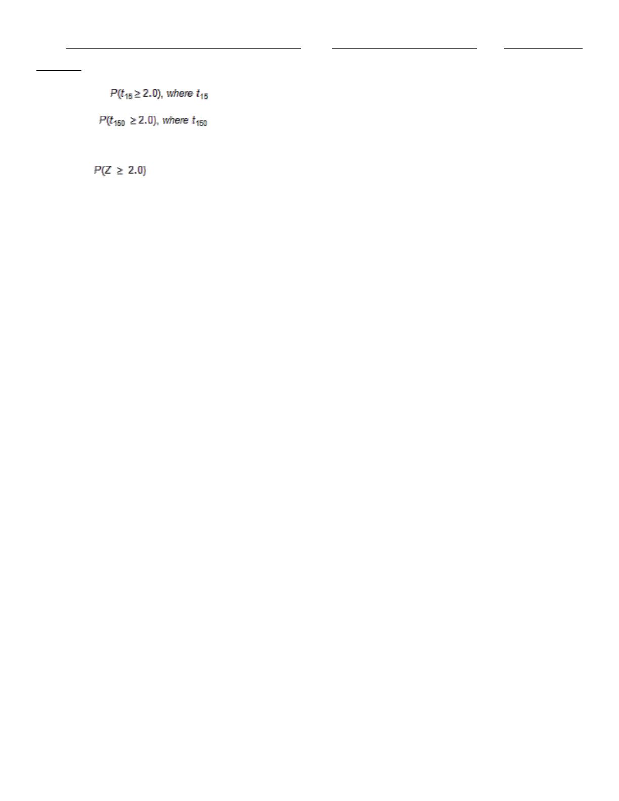
66. (A) Compute has a t-distribution with 15 degrees of freedom.
(B) Compute has a t-distribution with 150 degrees of freedom.
(C) How do you explain the difference between the results obtained in (A) and (B)?
(D) Compute where Z is a standard normal random variable.
(E) Compare the results of (D) to the results obtained in (A) and (B). How do you explain the difference in these
probabilities?
The personnel department of a large corporation wants to estimate the family dental expenses of its employees to
determine the feasibility of providing a dental insurance plan. A random sample of 12 employees in 2004 reveals the
following family dental expenses (in dollars): 115, 370, 250, 93, 540, 225, 177, 425, 318, 182, 275, and 228. Use
StatTools for your calculations.
67. (A) Construct a 90% confidence interval estimate of the mean family dental expenses for all employees of this
corporation.
(B) What assumption about the population distribution must be made to answer (A)?
(C) Interpret the 90% confidence interval constructed in (A).
(D) Suppose you used a 95% confidence interval in (A). What would be your answer?
(E) Suppose the fourth value were 593 instead of 93. What would be your answer to (A)? What effect does this change
have on the confidence interval?
(F) Construct a 90% confidence interval estimate for the standard deviation of family dental expenses for all employees of
this corporation.
(G) Interpret the 90% confidence interval constructed in (E).
A department store is interested in the average balance that is carried on its store’s credit card. A sample of 40 accounts
reveals an average balance of $1,250 and a standard deviation of $350.
68. (A) Find a 95% confidence interval for the mean account balance on this store’s credit card (the t–multiple with 39
degrees of freedom is 2.0227).
(B) What sample size would be needed to ensure that we could estimate the true mean account balance and have only 5
chances in 100 of being off by more than $100?
The employee benefits manager of a medium size business would like to estimate the proportion of full-time employees
who prefer adopting plan A of three available health care plans in the coming annual enrollment period. A reliable frame of
the company’s employees and their tentative health care preferences are available. Using Excel, the manager chose a
random sample of size 50 from the frame. There were 17 employees in the sample who preferred plan A.
69. (A) Construct a 99% confidence interval for the proportion of company employees who prefer plan A. Assume that the
population consists of the preferences of all employees in the frame.
(B) Interpret the 99% confidence interval constructed in (A).
Senior management of a consulting services firm is concerned about a growing decline in the firm’s weekly number of
billable hours. The firm expects each professional employee to spend at least 40 hours per week on work. In an effort to
understand this problem better, management would like to estimate the standard deviation of the number of hours their
employees spend on work-related activities in a typical week. Rather than reviewing the records of all the firm’s full-time
Name:
Class:
Date:
chapter 8
employees, the management randomly selected a sample of size 50 from the available frame. The sample mean and
sample standard deviations were 48.5 and 7.5 hours, respectively.
70. (A) Construct a 99% confidence interval for the standard deviation of the number of hours this firm’s employees spend
on work-related activities in a typical week.
(B) Interpret the 99% confidence interval constructed in (A).
(C) Given the target range of 40 to 60 hours of work per week, should senior management be concerned about the
number of hours their employees are currently devoting to work? Explain why or why not.
71. You are trying to estimate the average amount a family spends on food during a year. In the past, the standard
deviation of the amount a family has spent on food during a year has been approximately $1200. If you want to be 99%
sure that you have estimated average family food expenditures within $60, how many families do you need to survey?
The following values have been calculated using the TDIST and TINV functions in Excel. These values come from a t-
distribution with 15 degrees of freedom.
These values represent the probability to the right of the given positive values.
Value
t -probability
1.00
0.1666
1.20
0.1244
1.40
0.0909
These values represent the positive t- value for a given probability in both tails (sum of both tails).
Probability
t -value
0.20
1.3406
0.10
1.7531
0.05
2.1315
72. What is the probability of a t-value smaller than 1.00?
73. What would be the t-value where 0.05 of the values are in the upper tail?
74. In past years, approximately 25% of all U.S. families purchased potato chips at least once a month. We are interested
in determining the fraction of all U.S. families that currently purchase potato chips at least once a month. How many
families must we survey if we want to be 99% sure that our estimate of the fraction of U.S. families currently purchasing
potato chips at least once a month is accurate within 2%?
The following values have been calculated using the TDIST and TINV functions in Excel. These values come from a t-
distribution with 15 degrees of freedom.
These values represent the probability to the right of the given positive values.
Value
t -probability
1.00
0.1666
1.20
0.1244
1.40
0.0909
These values represent the positive t- value for a given probability in both tails (sum of both tails).
Probability
t -value
0.20
1.3406
0.10
1.7531
0.05
2.1315
75. What would be the t-values where 0.10 of the values are in both tails (sum of both tails)?
Name:
Class:
Date:
chapter 8
A market research consultant hired by Coke Classic Company is interested in estimating the difference between the
proportions of female and male customers who favor Coke Classic over Pepsi Cola in Chicago. A random sample of 200
consumers from the market under investigation showed the following frequency distribution.
Male
Female
Coke
72
38
110
Pepsi
58
32
90
130
70
200
76. (A) Construct a 95% confidence interval for the difference between the proportions of male and female customers who
prefer Coke Classic over Pepsi Cola.
(B) Interpret the constructed confidence interval.
The following values have been calculated using the TDIST and TINV functions in Excel. These values come from a t-
distribution with 15 degrees of freedom.
These values represent the probability to the right of the given positive values.
Value
t -probability
1.00
0.1666
1.20
0.1244
1.40
0.0909
These values represent the positive t- value for a given probability in both tails (sum of both tails).
Probability
t -value
0.20
1.3406
0.10
1.7531
0.05
2.1315
77. What is the probability of a t-value between –1.40 and +1.40?
78. In constructing confidence interval estimate for the difference between the means of two populations, where the
unknown population variances are assumed not to be equal, summary statistics computed from two independent samples
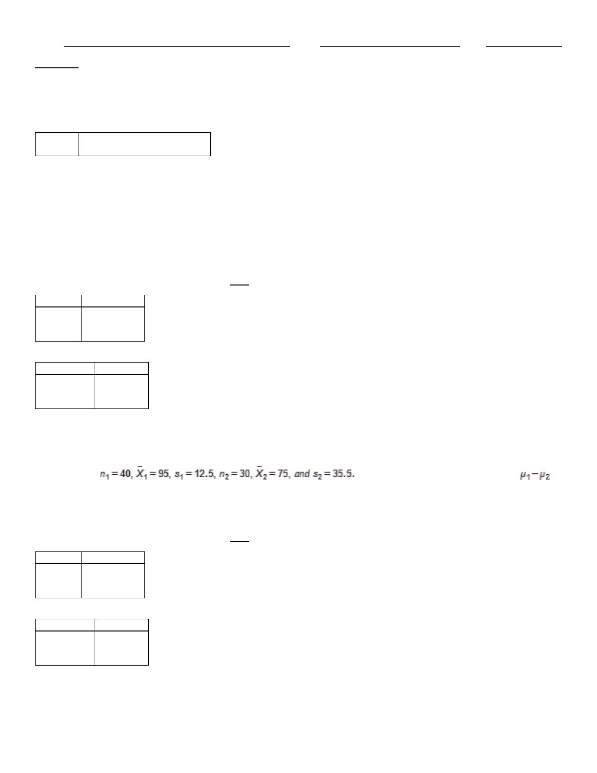
are as follows: Construct 90% confidence interval for .
The following values have been calculated using the TDIST and TINV functions in Excel. These values come from a t-
distribution with 15 degrees of freedom.
These values represent the probability to the right of the given positive values.
Value
t -probability
1.00
0.1666
1.20
0.1244
1.40
0.0909
These values represent the positive t- value for a given probability in both tails (sum of both tails).
Probability
t -value
0.20
1.3406
0.10
1.7531
0.05
2.1315
79. What would be the t-values where 0.95 of the values would fall within this interval?
Auditors of Independent Bank are interested in comparing the reported value of all 1775 customer savings account
balances with their own findings regarding the actual value of such assets. Rather than reviewing the records of each
Name:
Class:
Date:
chapter 8
savings account at the bank, the auditors randomly selected a sample of 100 savings account balances from the frame.
The sample mean and sample standard deviations were $505.75 and 360.95, respectively.
80. (A) Construct a 90% confidence interval for the total value of all savings account balances within this bank. Assume
that the population consists of all savings account balances in the frame.
(B) Interpret the 90% confidence interval constructed in (A).
A sample of 9 production managers with over 15 years of experience has an average salary of $71,000 and a sample
standard deviation of $18,000.
81. (A) You can be 95% confident that the mean salary for all production managers with at least 15 years of experience is
between what two numbers (the t-multiple with 8 degrees of freedom is 2.306)? What assumption are you making about
the distribution of salaries?
(B) What sample size would be needed to ensure that we could estimate the true mean salary of all production managers
with more than 15 years of experience and have only 5 chances in 100 of being off by more than $4200?
The widths of 100 elevator rails have been measured. The sample mean and standard deviation of the elevator rails are
2.05 inches and 0.01 inch.
82. (A) Construct a 95% confidence interval for the average width of an elevator rail. Do we need to assume that the width
of elevator rails follows a normal distribution?
(B) How large a sample of elevator rails would we have to measure to ensure that we could estimate, with 95%
confidence, the average diameter of an elevator rail within 0.01 inch?
An automobile dealer wants to estimate the proportion of customers who still own the cars they purchased six years ago.
A random sample of 200 customers selected from the automobile dealer’s records indicates that 88 still own cars that
were purchased six years earlier.
83. (A) Construct a 95% confidence interval estimate of the population proportion of all customers who still own the cars
they purchased six years ago
(B) How can the result in (A) be used by the automobile dealer to study satisfaction with cars purchased at the
dealership?
84. You are told that a random sample of 150 people from Iowa has been given cholesterol tests, and 60 of these people
had levels over the “safe” count of 200. Construct a 95% confidence interval for the population proportion of people in
Iowa with cholesterol levels over 200.
A defensive driving training company is interested in evaluating the relative effectiveness of its two main modes of
training; online and traditional classroom. The company has collected a random sample of 300 customers in a particular
area, with the following results:
Online
Classroom
Pass
143
128
Fail
17
12
Total
160
140
85. (A) Construct a 95% confidence interval for the difference between the proportions of online and classroom customers
who pass the final exam.
(B) Interpret the confidence interval obtained in (A).
The following values have been calculated using the TDIST and TINV functions in Excel. These values come from a t-
distribution with 15 degrees of freedom.
Name:
Class:
Date:
chapter 8
These values represent the probability to the right of the given positive values.
Value
t -probability
1.00
0.1666
1.20
0.1244
1.40
0.0909
These values represent the positive t- value for a given probability in both tails (sum of both tails).
Probability
t -value
0.20
1.3406
0.10
1.7531
0.05
2.1315
86. What is the probability of a t-value larger than 1.20?
Name:
Class:
Date:
chapter 8
Answer Key
Name:
Class:
Date:
chapter 8
Name:
Class:
Date:
chapter 8
Name:
Class:
Date:
chapter 8
Name:
Class:
Date:
chapter 8
City
Household
City
Household
City
Household
Income
Income
Income
1
$54,300
$53,500
$61,500
2
$61,800
$45,600
$53,000
3
$61,400
$70,100
$51,000
4
$50,800
$108,700
$55,600
5
$56,200
$46,400
$51,600
6
$48,300
$56,700
$57,200
7
$61,600
$59,100
$54,300
8
$63,200
$46,300
$51,500
9
$55,200
$52,900
$53,500
$58,000
$56,300
$61,800
$77,600
$67,300
$44,800
$47,600
$63,800
$57,400
$62,700
$70,600
$48,100
$46,200
$49,800
$52,700
$64,300
$51,300
$57,400
$56,000
$56,600
$65,500
$53,400
$49,600
$59,600
$56,800
$67,400
$62,000
$51,200
$53,700
$49,700
$59,000
$48,700
$54,400
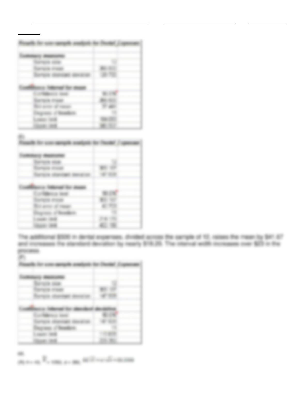
(C) We are 95% confident that the average annual household income level of all citizens is approximately between
Name:
Class:
Date:
chapter 8
intervals constructed in this way should contain the true population mean.
(D)
Name:
Class:
Date:
chapter 8
Name:
Class:
Date:
chapter 8
0.8334
+ 1.7531
Name:
Class:
Date:
chapter 8
– 1.7531 and + 1.7531
0.8182
– 2.1315 and + 2.1315
Name:
Class:
Date:
chapter 8
0.1244