Chapter 7 If the expected value of a sample statistic is equal to the parameter

subject Type Homework Help
subject Pages 23
subject Words 6361
subject Authors David M. Levine, Kathryn A. Szabat, Mark L. Berenson

Unlock document.

This document is partially blurred.
Unlock all pages and 1 million more documents.
Get Access
page-pf1
Sampling Distributions 7-1
CHAPTER 7: SAMPLING DISTRIBUTIONS
1. Sampling distributions describe the distribution of
a) parameters.
b) statistics.
c) both parameters and statistics.
d) neither parameters nor statistics.
2. The standard error of the mean
a) is never larger than the standard deviation of the population.
b) decreases as the sample size increases.
c) measures the variability of the mean from sample to sample.
d) All of the above.
3. The Central Limit Theorem is important in statistics because
a) for a large n, it says the population is approximately normal.
b) for any population, it says the sampling distribution of the sample mean is approximately
normal, regardless of the sample size.
c) for a large n, it says the sampling distribution of the sample mean is approximately
normal, regardless of the shape of the population.
d) for any sized sample, it says the sampling distribution of the sample mean is
approximately normal.
4. If the expected value of a sample statistic is equal to the parameter it is estimating, then we call
that sample statistic
a) unbiased.
b) minimum variance.
c) biased.
d) random.
page-pf2
7-2 Sampling Distributions
5. For air travelers, one of the biggest complaints is of the waiting time between when the airplane
taxis away from the terminal until the flight takes off. This waiting time is known to have a right
skewed distribution with a mean of 10 minutes and a standard deviation of 8 minutes. Suppose
100 flights have been randomly sampled. Describe the sampling distribution of the mean waiting
time between when the airplane taxis away from the terminal until the flight takes off for these
100 flights.
a) Distribution is right skewed with mean = 10 minutes and standard error = 0.8 minutes.
b) Distribution is right skewed with mean = 10 minutes and standard error = 8 minutes.
c) Distribution is approximately normal with mean = 10 minutes and standard error = 0.8
minutes.
d) Distribution is approximately normal with mean = 10 minutes and standard error = 8
minutes.
6. Which of the following statements about the sampling distribution of the sample mean is
incorrect?
a) The sampling distribution of the sample mean is approximately normal whenever the
sample size is sufficiently large (n30 ).
b) The sampling distribution of the sample mean is generated by repeatedly taking samples
of size n and computing the sample means.
c) The mean of the sampling distribution of the sample mean is equal to
μ
.
d) The standard deviation of the sampling distribution of the sample mean is equal to
σ
.
7. Which of the following is true about the sampling distribution of the sample mean?
a) The mean of the sampling distribution is always
μ
.
b) The standard deviation of the sampling distribution is always
σ
.
c) The shape of the sampling distribution is always approximately normal.
d) All of the above are true.
page-pf3
Sampling Distributions 7-3
8. True or False: The amount of time it takes to complete an examination has a left skewed
distribution with a mean of 65 minutes and a standard deviation of 8 minutes. If 64 students were
randomly sampled, the probability that the sample mean of the sampled students exceeds 71
minutes is approximately 0.
9. Suppose the ages of students in Statistics 101 follow a right skewed distribution with a mean of
23 years and a standard deviation of 3 years. If we randomly sampled 100 students, which of the
following statements about the sampling distribution of the sample mean age is incorrect?
a) The mean of the sampling distribution is equal to 23 years.
b) The standard deviation of the sampling distribution is equal to 3 years.
c) The shape of the sampling distribution is approximately normal.
d) The standard error of the sampling distribution is equal to 0.3 years.
10. Why is the Central Limit Theorem so important to the study of sampling distributions?
a) It allows us to disregard the size of the sample selected when the population is not
normal.
b) It allows us to disregard the shape of the sampling distribution when the size of the
population is large.
c) It allows us to disregard the size of the population we are sampling from.
d) It allows us to disregard the shape of the population when n is large.
11. A sample that does not provide a good representation of the population from which it was
collected is referred to as a(n) sample.
page-pf4
7-4 Sampling Distributions
12. True or False: The Central Limit Theorem is considered powerful in statistics because it works
for any population distribution provided the sample size is sufficiently large and the population
mean and standard deviation are known.
13. Suppose a sample of n = 50 items is selected from a population of manufactured products and the
weight, X, of each item is recorded. Prior experience has shown that the weight has a probability
distribution with
μ
= 6 ounces and
σ
= 2.5 ounces. Which of the following is true about the
sampling distribution of the sample mean if a sample of size 15 is selected?
a) The mean of the sampling distribution is 6 ounces.
b) The standard deviation of the sampling distribution is 2.5 ounces.
c) The shape of the sampling distribution is approximately normal.
d) All of the above are correct.
14. The mean score of all pro golfers for a particular course has a mean of 70 and a standard
deviation of 3.0. Suppose 36 pro golfers played the course today. Find the probability that the
mean score of the 36 pro golfers exceeded 71.
15. The distribution of the number of loaves of bread sold per week by a large bakery over the past 5
years has a mean of 7,750 and a standard deviation of 145 loaves. Suppose a random sample of n
= 40 weeks has been selected. What is the approximate probability that the mean number of
loaves sold in the sampled weeks exceeds 7,895 loaves?
page-pf5
Sampling Distributions 7-5
16. Sales prices of baseball cards from the 1960s are known to possess a right skewed distribution
with a mean sale price of $5.25 and a standard deviation of $2.80. Suppose a random sample of
100 cards from the 1960s is selected. Describe the sampling distribution for the sample mean sale
price of the selected cards.
a) Right skewed with a mean of $5.25 and a standard error of $2.80
b) Normal with a mean of $5.25 and a standard error of $0.28
c) Right skewed with a mean of $5.25 and a standard error of $0.28
d) Normal with a mean of $5.25 and a standard error of $2.80
17. Major league baseball salaries averaged $3.26 million with a standard deviation of $1.2 million in
a certain year in the past. Suppose a sample of 100 major league players was taken. What was the
standard error for the sample mean salary?
a) $0.012 million
b) $0.12 million
c) $12 million
d) $1,200.0 million
18. Major league baseball salaries averaged $3.26 million with a standard deviation of $1.2 million in
a certain year in the past. Suppose a sample of 100 major league players was taken. Find the
approximate probability that the mean salary of the 100 players exceeded $3.5 million.
a) Approximately 0
b) 0.0228
c) 0.9772
d) Approximately 1
page-pf6
7-6 Sampling Distributions
19. Major league baseball salaries averaged $3.26 million with a standard deviation of $1.2 million in
a certain year in the past. Suppose a sample of 100 major league players was taken. Find the
approximate probability that the mean salary of the 100 players exceeded $4.0 million.
a) Approximately 0
b) 0.0228
c) 0.9772
d) Approximately 1
20. Major league baseball salaries averaged $3.26 million with a standard deviation of $1.2 million in
a certain year in the past. Suppose a sample of 100 major league players was taken. Find the
approximate probability that the mean salary of the 100 players was no more than $3.0 million.
a) Approximately 0
b) 0.0151
c) 0.9849
d) Approximately 1
21. Major league baseball salaries averaged $3.26 million with a standard deviation of $1.2 million in
a certain year in the past. Suppose a sample of 100 major league players was taken. Find the
approximate probability that the mean salary of the 100 players was less than $2.5 million.
a) Approximately 0
b) 0.0151
c) 0.9849
d) Approximately 1
page-pf7
Sampling Distributions 7-7
22. At a computer manufacturing company, the actual size of a particular type of computer chips is
normally distributed with a mean of 1 centimeter and a standard deviation of 0.1 centimeter. A
random sample of 12 computer chips is taken. What is the standard error for the sample mean?
a) 0.029
b) 0.050
c) 0.091
d) 0.120
23. At a computer manufacturing company, the actual size of a particular type of computer chips is
normally distributed with a mean of 1 centimeter and a standard deviation of 0.1 centimeter. A
random sample of 12 computer chips is taken. What is the probability that the sample mean will
be between 0.99 and 1.01 centimeters?
24. At a computer manufacturing company, the actual size of a particular type of computer chips is
normally distributed with a mean of 1 centimeter and a standard deviation of 0.1 centimeter. A
random sample of 12 computer chips is taken. What is the probability that the sample mean will
be below 0.95 centimeters?
25. At a computer manufacturing company, the actual size of a particular type of computer chips is
normally distributed with a mean of 1 centimeter and a standard deviation of 0.1 centimeter. A
random sample of 12 computer chips is taken. Above what value do 2.5% of the sample means
fall?
page-pf8
7-8 Sampling Distributions
26. The owner of a fish market has an assistant who has determined that the weights of catfish are
normally distributed, with mean of 3.2 pounds and standard deviation of 0.8 pound. If a sample of
16 fish is taken, what would the standard error of the mean weight equal?
a) 0.003
b) 0.050
c) 0.200
d) 0.800
27. The owner of a fish market has an assistant who has determined that the weights of catfish are
normally distributed, with mean of 3.2 pounds and standard deviation of 0.8 pound. If a sample of
25 fish yields a mean of 3.6 pounds, what is the Z-score for this observation?
a) 18.750
b) 2.500
c) 1.875
d) 0.750
28. The owner of a fish market has an assistant who has determined that the weights of catfish are
normally distributed, with mean of 3.2 pounds and standard deviation of 0.8 pound. If a sample of
64 fish yields a mean of 3.4 pounds, what is probability of obtaining a sample mean this large or
larger?
a) 0.0001
b) 0.0013
c) 0.0228
d) 0.4987
page-pf9
Sampling Distributions 7-9
29. The owner of a fish market has an assistant who has determined that the weights of catfish are
normally distributed, with mean of 3.2 pounds and standard deviation of 0.8 pound. What
percentage of samples of 4 fish will have sample means between 3.0 and 4.0 pounds?
a) 84%
b) 67%
c) 29%
d) 16%
30. For sample size 16, the sampling distribution of the mean will be approximately normally
distributed
a) regardless of the shape of the population.
b) if the shape of the population is symmetrical.
c) if the sample standard deviation is known.
d) if the sample is normally distributed.
31. The standard error of the mean for a sample of 100 is 30. In order to cut the standard error of the
mean to 15, we would
a) increase the sample size to 200.
b) increase the sample size to 400.
c) decrease the sample size to 50.
d) decrease the sample to 25.
32. Which of the following is true regarding the sampling distribution of the mean for a large sample
size?
a) It has the same shape, mean, and standard deviation as the population.
b) It has a normal distribution with the same mean and standard deviation as the population.
c) It has the same shape and mean as the population, but has a smaller standard deviation.
d) It has a normal distribution with the same mean as the population but with a smaller
standard deviation.
page-pfa
7-10 Sampling Distributions
33. For sample sizes greater than 30, the sampling distribution of the mean will be approximately
normally distributed
a) regardless of the shape of the population.
b) only if the shape of the population is symmetrical.
c) only if the standard deviation of the samples are known.
d) only if the population is normally distributed.
34. For sample size 1, the sampling distribution of the mean will be normally distributed
a) regardless of the shape of the population.
b) only if the shape of the population is symmetrical.
c) only if the population values are positive.
d) only if the population is normally distributed.
35. The standard error of the population proportion will become larger
a) as population proportion approaches 0.
b) as population proportion approaches 0.50.
c) as population proportion approaches 1.00.
d) as the sample size increases.
36. True or False: As the sample size increases, the standard error of the mean increases.
37. True or False: If the population distribution is symmetric, the sampling distribution of the mean
can be approximated by the normal distribution if the samples contain 15 observations.
page-pfb
Sampling Distributions 7-11
38. True or False: If the population distribution is unknown, in most cases the sampling distribution
of the mean can be approximated by the normal distribution if the samples contain at least 30
observations.
39. True or False: If the amount of gasoline purchased per car at a large service station has a
population mean of 15 gallons and a population standard deviation of 4 gallons, then 99.73% of
all cars will purchase between 3 and 27 gallons.
40. True or False: If the amount of gasoline purchased per car at a large service station has a
population mean of 15 gallons and a population standard deviation of 4 gallons and a random
sample of 4 cars is selected, there is approximately a 68.26% chance that the sample mean will be
between 13 and 17 gallons.
41. True or False: If the amount of gasoline purchased per car at a large service station has a
population mean of 15 gallons and a population standard deviation of 4 gallons and it is assumed
that the amount of gasoline purchased per car is symmetric, there is approximately a 68.26%
chance that a random sample of 16 cars will have a sample mean between 14 and 16 gallons.
42. True or False: If the amount of gasoline purchased per car at a large service station has a
population mean of 15 gallons and a population standard deviation of 4 gallons and a random
sample of 64 cars is selected, there is approximately a 95.44% chance that the sample mean will
be between 14 and 16 gallons.
page-pfc
7-12 Sampling Distributions
43. True or False: As the sample size increases, the effect of an extreme value on the sample mean
becomes smaller.
44. True or False: If the population distribution is skewed, in most cases the sampling distribution
of the mean can be approximated by the normal distribution if the samples contain at least 30
observations.
45. True or False: A sampling distribution is a distribution for a statistic.
46. True or False: Suppose
μ
= 50 and
σ
= 10 for a population. In a sample where n = 100 is
randomly taken, 95% of all possible sample means will fall between 48.04 and 51.96.
47. True or False: Suppose
μ
= 80 and
σ
= 20 for a population. In a sample where n = 100 is
randomly taken, 95% of all possible sample means will fall above 76.71.
48. True or False: Suppose
μ
= 50 and
σ
= 10 for a population. In a sample where n = 100 is
randomly taken, 90% of all possible sample means will fall between 49 and 51.
page-pfd
Sampling Distributions 7-13
49. True or False: The Central Limit Theorem ensures that the sampling distribution of the sample
mean approaches a normal distribution as the sample size increases.
50. True or False: The standard error of the mean is also known as the standard deviation of the
sampling distribution of the sample mean.
51. True or False: A sampling distribution is defined as the probability distribution of possible
sample sizes that can be observed from a given population.
52. True or False: As the size of the sample is increased, the standard deviation of the sampling
distribution of the sample mean for a normally distributed population will stay the same.
53. True or False: For distributions such as the normal distribution, the arithmetic mean is
considered more stable from sample to sample than other measures of central tendency.
54. True or False: The fact that the sample means are less variable than the population data can be
observed from the standard error of the mean.
page-pfe
7-14 Sampling Distributions
55. The amount of tea leaves in a can from a particular production line is normally distributed with
μ
= 110 grams and
σ
= 25 grams. A sample of 25 cans is to be selected. What is the probability
that the sample mean will be between 100 and 120 grams?
56. The amount of tea leaves in a can from a particular production line is normally distributed with
μ
= 110 grams and
σ
= 25 grams. A sample of 25 cans is to be selected. What is the
probability that the sample mean will be less than 100 grams?
57. The amount of tea leaves in a can from a particular production line is normally distributed with
μ
= 110 grams and
σ
= 25 grams. A sample of 25 cans is to be selected. What is the probability
that the sample mean will be greater than 100 grams?
58. The amount of tea leaves in a can from a particular production line is normally distributed with
μ
= 110 grams and
σ
= 25 grams. A sample of 25 cans is to be selected. So, 95% of all sample
means will be greater than how many grams?
59. The amount of tea leaves in a can from a particular production line is normally distributed with
μ
= 110 grams and
σ
= 25 grams. A sample of 25 cans is to be selected. So, the middle 70% of
all sample means will fall between what two values?
page-pff
Sampling Distributions 7-15
60. The amount of time required for an oil and filter change on an automobile is normally
distributed with a mean of 45 minutes and a standard deviation of 10 minutes. A random sample
of 16 cars is selected. What is the standard error of the mean?
61. The amount of time required for an oil and filter change on an automobile is normally
distributed with a mean of 45 minutes and a standard deviation of 10 minutes. A random sample
of 16 cars is selected. What is the probability that the sample mean is between 45 and 52
minutes?
62. The amount of time required for an oil and filter change on an automobile is normally
distributed with a mean of 45 minutes and a standard deviation of 10 minutes. A random sample
of 16 cars is selected. What is the probability that the sample mean will be between 39 and 48
minutes?
63. The amount of time required for an oil and filter change on an automobile is normally
distributed with a mean of 45 minutes and a standard deviation of 10 minutes. A random sample
of 16 cars is selected. 95% of all sample means will fall between what two values?
64. The amount of time required for an oil and filter change on an automobile is normally
distributed with a mean of 45 minutes and a standard deviation of 10 minutes. A random sample
of 16 cars is selected. 90% of the sample means will be greater than what value?
page-pf10
7-16 Sampling Distributions
65. True or False: The amount of bleach a machine pours into bottles has a mean of 36 oz. with a
standard deviation of 0.15 oz. Suppose we take a random sample of 36 bottles filled by this
machine. The sampling distribution of the sample mean has a mean of 36 oz.
66. True or False: The amount of bleach a machine pours into bottles has a mean of 36 oz. with a
standard deviation of 0.15 oz. Suppose we take a random sample of 36 bottles filled by this
machine. The sampling distribution of the sample mean has a standard error of 0.15.
67. True or False: The amount of bleach a machine pours into bottles has a mean of 36 oz. with a
standard deviation of 0.15 oz. Suppose we take a random sample of 36 bottles filled by this
machine. The sampling distribution of the sample mean will be approximately normal only if the
population sampled is normal.
68. The amount of bleach a machine pours into bottles has a mean of 36 oz. with a standard
deviation of 0.15 oz. Suppose we take a random sample of 36 bottles filled by this machine. The
probability that the mean of the sample exceeds 36.01 oz. is __________.
69. The amount of bleach a machine pours into bottles has a mean of 36 oz. with a standard
deviation of 0.15 oz. Suppose we take a random sample of 36 bottles filled by this machine. The
probability that the mean of the sample is less than 36.03 is __________.
page-pf11
Sampling Distributions 7-17
70. The amount of bleach a machine pours into bottles has a mean of 36 oz. with a standard
deviation of 0.15 oz. Suppose we take a random sample of 36 bottles filled by this machine. The
probability that the mean of the sample is between 35.94 and 36.06 oz. is __________.
71. The amount of bleach a machine pours into bottles has a mean of 36 oz. with a standard
deviation of 0.15 oz. Suppose we take a random sample of 36 bottles filled by this machine. The
probability that the mean of the sample is between 35.95 and 35.98 oz. is __________.
72. The amount of bleach a machine pours into bottles has a mean of 36 oz. with a standard
deviation of 0.15 oz. Suppose we take a random sample of 36 bottles filled by this machine. So,
the middle 95% of the sample means based on samples of size 36 will be between __________
and __________.
73. A manufacturer of power tools claims that the mean amount of time required to assemble their
top-of-the-line table saw is 80 minutes with a standard deviation of 40 minutes. Suppose a
random sample of 64 purchasers of this table saw is taken. The mean of the sampling distribution
of the sample mean is __________ minutes.
74. A manufacturer of power tools claims that the mean amount of time required to assemble their
top-of-the-line table saw is 80 minutes with a standard deviation of 40 minutes. Suppose a
random sample of 64 purchasers of this table saw is taken. The standard deviation of the sampling
distribution of the sample mean is __________ minutes.
page-pf12
7-18 Sampling Distributions
75. A manufacturer of power tools claims that the mean amount of time required to assemble their
top-of-the-line table saw is 80 minutes with a standard deviation of 40 minutes. Suppose a
random sample of 64 purchasers of this table saw is taken. The probability that the sample mean
will be less than 82 minutes is __________.
76. A manufacturer of power tools claims that the mean amount of time required to assemble their
top-of-the-line table saw is 80 minutes with a standard deviation of 40 minutes. Suppose a
random sample of 64 purchasers of this table saw is taken. The probability that the sample mean
will be between 77 and 89 minutes is __________.
77. A manufacturer of power tools claims that the mean amount of time required to assemble their
top-of-the-line table saw is 80 minutes with a standard deviation of 40 minutes. Suppose a
random sample of 64 purchasers of this table saw is taken. The probability that the sample mean
will be greater than 88 minutes is __________.
78. A manufacturer of power tools claims that the mean amount of time required to assemble their
top-of-the-line table saw is 80 minutes with a standard deviation of 40 minutes. Suppose a
random sample of 64 purchasers of this table saw is taken. So, the middle 95% of the sample
means based on samples of size 64 will be between __________ and __________.
79. To use the normal distribution to approximate the binomial distribution, we need ______ and
______ to be at least 5.
page-pf13
Sampling Distributions 7-19
80. True or False: The sample mean is an unbiased estimate of the population mean.
81. True or False: The sample proportion is an unbiased estimate of the population proportion.
82. True or False: The mean of the sampling distribution of a sample proportion is the population
proportion,
π
.
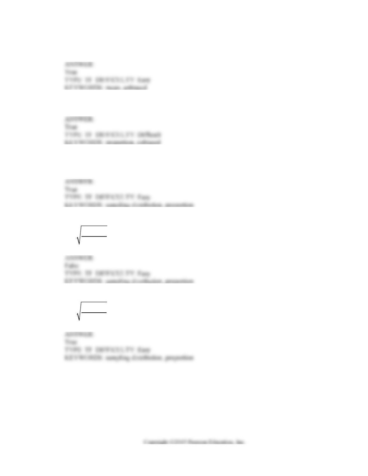
83. True or False: The standard error of the sampling distribution of a sample proportion is
()
1pp
n
where
is the sample proportion.
84. True or False: The standard deviation of the sampling distribution of a sample proportion is
()
1
n
ππ
where
π
is the population proportion.
page-pf14
7-20 Sampling Distributions
85. True or False: A sample of size 25 provides a sample variance of 400. The standard error, in
this case equal to 4, is best described as the estimate of the standard deviation of means calculated
from samples of size 25.
86. True or False: An unbiased estimator will have a value, on average across samples, equal to the
population parameter value.
87. True or False: In inferential statistics, the standard error of the sample mean assesses the
uncertainty or error of estimation.
88. True or False: The sample proportion is an unbiased estimator for the population proportion.
89. True or False: The sample mean is an unbiased estimator for the population mean.
90. Assume that house prices in a neighborhood are normally distributed with a standard deviation
of $20,000. A random sample of 16 observations is taken. What is the probability that the
sample mean differs from the population mean by more than $5,000?
page-pf15
Sampling Distributions 7-21
SCENARIO 7-1
The time spent studying by students in the week before final exams follows a normal distribution with
a standard deviation of 8 hours. A random sample of 4 students was taken in order to estimate the
mean study time for the population of all students.
91. Referring to Scenario 7-1, what is the probability that the sample mean exceeds the population
mean by more than 2 hours?
92. Referring to Scenario 7-1, what is the probability that the sample mean is more than 3 hours
below the population mean?
93. Referring to Scenario 7-1, what is the probability that the sample mean differs from the
population mean by less than 2 hours?
94. Referring to Scenario 7-1, what is the probability that the sample mean differs from the
population mean by more than 3 hours?
page-pf16
7-22 Sampling Distributions
SCENARIO 7-2
The mean selling price of new homes in a small town over a year was $115,000. The population
standard deviation was $25,000. A random sample of 100 new home sales from this city was taken.
95. Referring to Scenario 7-2, what is the probability that the sample mean selling price was more
than $110,000?
96. Referring to Scenario 7-2, what is the probability that the sample mean selling price was
between $113,000 and $117,000?
97. Referring to Scenario 7-2, what is the probability that the sample mean selling price was
between $114,000 and $116,000?
98. Referring to Scenario 7-2, without doing the calculations, state in which of the following ranges
the sample mean selling price is most likely to lie?
a) $113,000 -- $115,000
b) $114,000 -- $116,000
c) $115,000 -- $117,000
d) $116,000 -- $118,000
page-pf17
Sampling Distributions 7-23
SCENARIO 7-3
The lifetimes of a certain brand of light bulbs are known to be normally distributed with a mean of
1,600 hours and a standard deviation of 400 hours. A random sample of 64 of these light bulbs is
taken.
99. Referring to Scenario 7-3, what is the probability that the sample mean lifetime is more than
1,550 hours?
100. Referring to Scenario 7-3, the probability is 0.15 that the sample mean lifetime is more than
how many hours?
101. Referring to Scenario 7-3, the probability is 0.20 that the sample mean lifetime differs from the
population mean lifetime by at least how many hours?
SCENARIO 7-4
According to a survey, only 15% of customers who visited the web site of a major retail store made a
purchase. Random samples of size 50 are selected.
102. Referring to Scenario 7-4, the mean of all the sample proportions of customers who will make a
purchase after visiting the web site is _______.
page-pf18
7-24 Sampling Distributions
103. Referring to Scenario 7-4, the standard deviation of all the sample proportions of customers
who will make a purchase after visiting the web site is ________.
104. True or False: Referring to Scenario 7-4, the requirements for using a normal distribution to
approximate a binomial distribution is fulfilled.
105. Referring to Scenario 7-4, what proportion of the samples will have between 20% and 30% of
customers who will make a purchase after visiting the web site?
106. Referring to Scenario 7-4, what proportion of the samples will have less than 15% of customers
who will make a purchase after visiting the web site?
107. Referring to Scenario 7-4, what is the probability that a random sample of 50 will have at least
30% of customers who will make a purchase after visiting the web site?
108. Referring to Scenario 7-4, 90% of the samples will have less than what percentage of customers
who will make a purchase after visiting the web site?
page-pf19
Sampling Distributions 7-25
109. Referring to Scenario 7-4, 90% of the samples will have more than what percentage of
customers who will make a purchase after visiting the web site?
110. A study at a college in the west coast reveals that, historically, 45% of the students are minority
students. The expected percentage of minority students in their next group of freshmen is
_______.
111. A study at a college in the west coast reveals that, historically, 45% of the students are minority
students. If random samples of size 75 are selected, the standard error of the proportion of
students in the samples who are minority students is _________.
112. A study at a college in the west coast reveals that, historically, 45% of the students are minority
students. If a random sample of size 75 is selected, the probability is _______ that between 30%
and 50% of the students in the sample will be minority students.
113. A study at a college in the west coast reveals that, historically, 45% of the students are minority
students. If a random sample of size 75 is selected, the probability is _______ that more than half
of the students in the sample will be minority students.
page-pf1a
7-26 Sampling Distributions
114. A study at a college in the west coast reveals that, historically, 45% of the students are minority
students. If random samples of size 75 are selected, 80% of the samples will have less than
______% of minority students.
115. A study at a college in the west coast reveals that, historically, 45% of the students are minority
students. If random samples of size 75 are selected, 95% of the samples will have more than
______% of minority students.
SCENARIO 7-5
According to an article, 19% of the entire population in a developing country have high-speed access
to the Internet. Random samples of size 200 are selected from the country’s population.
116. Referring to Scenario 7-5, the population mean of all the sample proportions is ______.
117. Referring to Scenario 7-5, the standard error of all the sample proportions is ______.
118. Referring to Scenario 7-5, among all the random samples of size 200, ______ % will have
between 14% and 24% who have high-speed access to the Internet.
page-pf1b
Sampling Distributions 7-27
119. Referring to Scenario 7-5, among all the random samples of size 200, ______ % will have
between 9% and 29% who have high-speed access to the Internet.
120. Referring to Scenario 7-5, among all the random samples of size 200, ______ % will have more
than 30% who have high-speed access to the Internet.
121. Referring to Scenario 7-5, among all the random samples of size 200, ______ % will have less
than 20% who have high-speed access to the Internet.
122. Referring to Scenario 7-5, among all the random samples of size 200, 90 % will have less than
_____% who have high-speed access to the Internet.
123. Referring to Scenario 7-5, among all the random samples of size 200, 90 % will have more than
_____% who have high-speed access to the Internet.
page-pf1c
7-28 Sampling Distributions
SCENARIO 7-6
Online customer service is a key element to successful online retailing. According to a marketing
survey, 37.5% of online customers take advantage of the online customer service. Random samples
of 200 customers are selected.
124. Referring to Scenario 7-6, the population mean of all possible sample proportions is ______.
125. Referring to Scenario 7-6, the standard error of all possible sample proportions is ______.
126. Referring to Scenario 7-6, ____ % of the samples are likely to have between 35% and 40% who
take advantage of online customer service.
127. Referring to Scenario 7-6, ____ % of the samples are likely to have less than 37.5% who take
advantage of online customer service.
128. Referring to Scenario 7-6, 90% of the samples proportions symmetrically around the population
proportion will have between _____% and _____% of the customers who take advantage of
online customer service.
page-pf1d
Sampling Distributions 7-29
129. Referring to Scenario 7-6, 95% of the samples proportions symmetrically around the population
proportion will have between _____% and _____% of the customers who take advantage of
online customer service.

Trusted by Thousands of
Students

Here are what students say about us.

Copyright ©2022 All rights reserved. | CoursePaper is not sponsored or endorsed by any college or university.