Chapter 7
1.
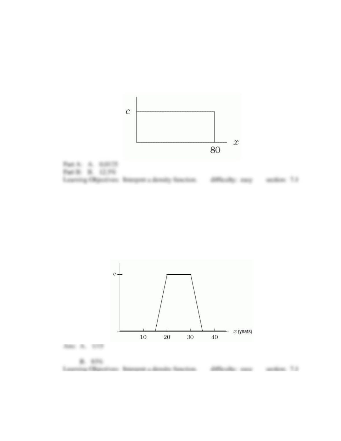
A density function for the daily calorie intake of a certain species is given in the
following figure.
A. Find the value of c.
B. What percent have daily calorie intake between 30 and 40?
2.
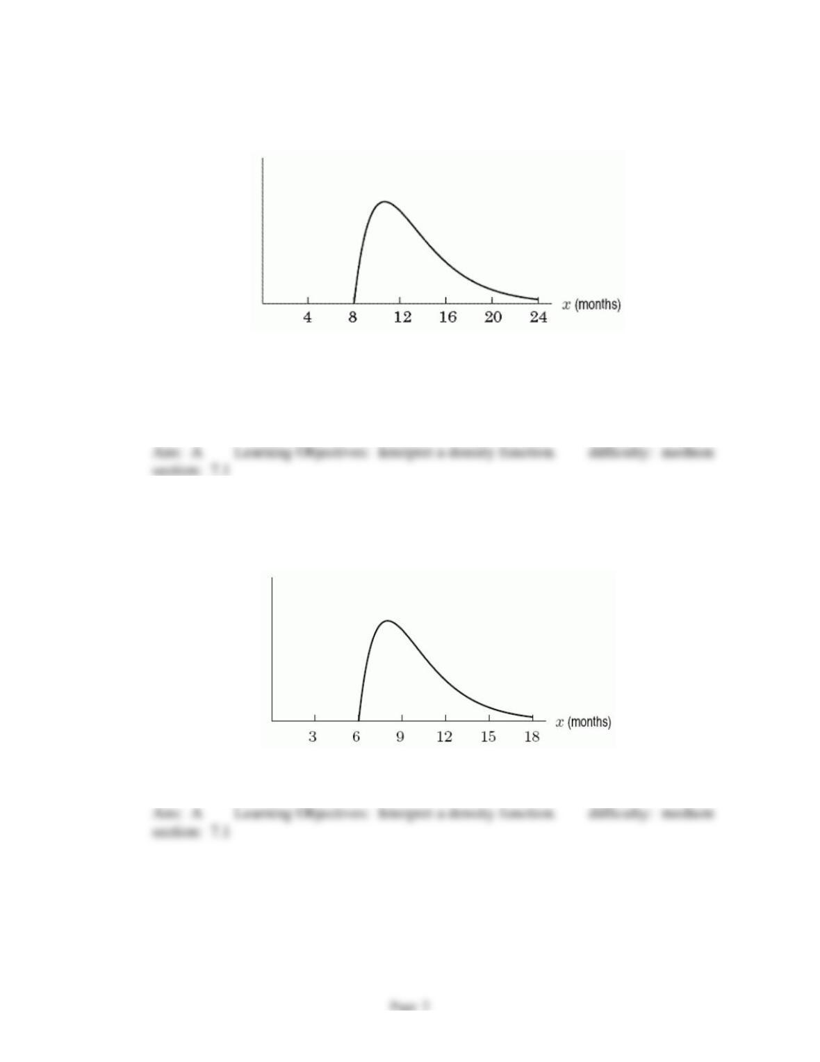
A density function for the age of people enrolled in a class is given in the following
figure.
A. Find the value of c.
B. What percent of the class is over 20 years old? Round to the nearest whole
percent.
Chapter 7
3.
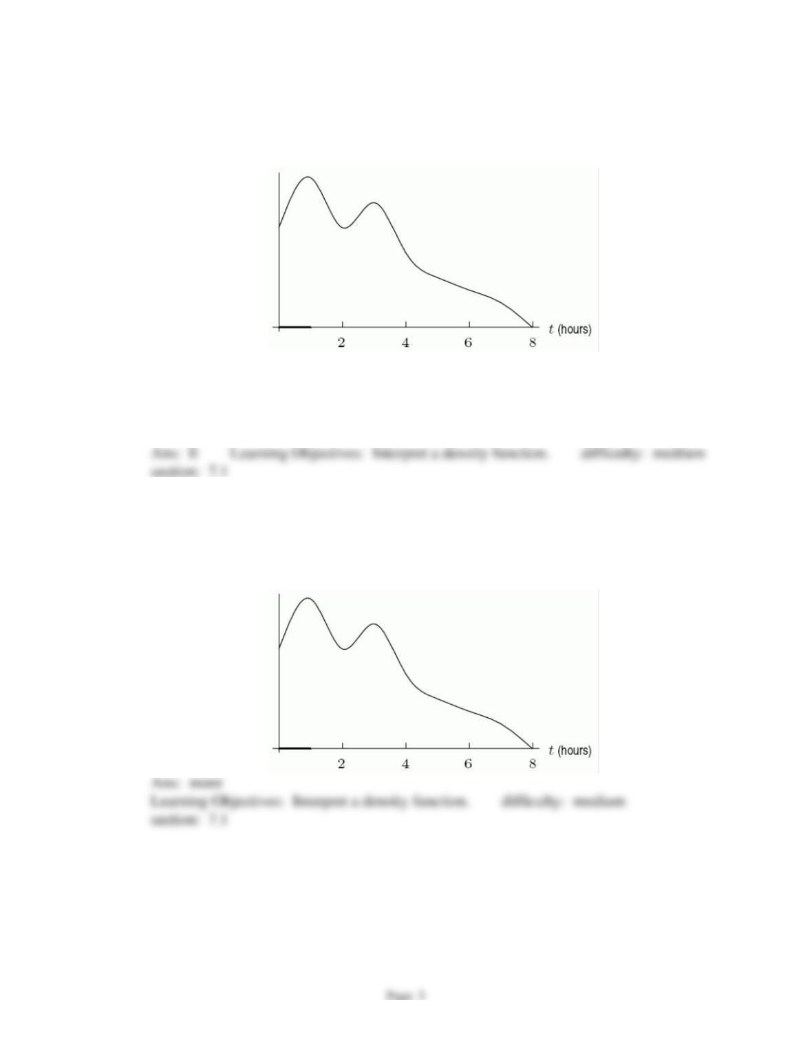
A density function for the lifetime of a certain type of frog is shown in the following
figure. What is the most likely lifetime for a frog of this type?
A)
11 months
B)
14 months
C)
16 months
D)
19 months
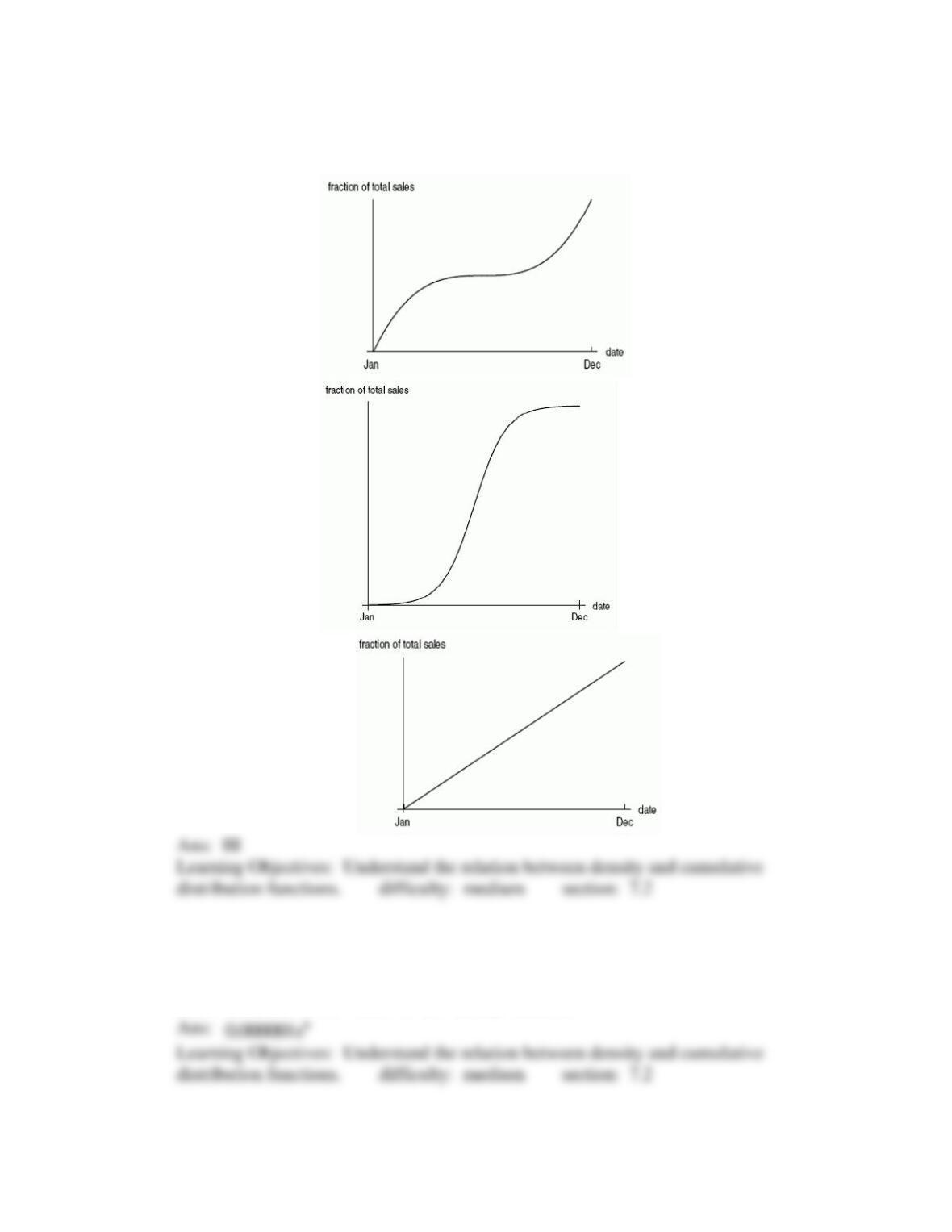
E)
21 months
F)
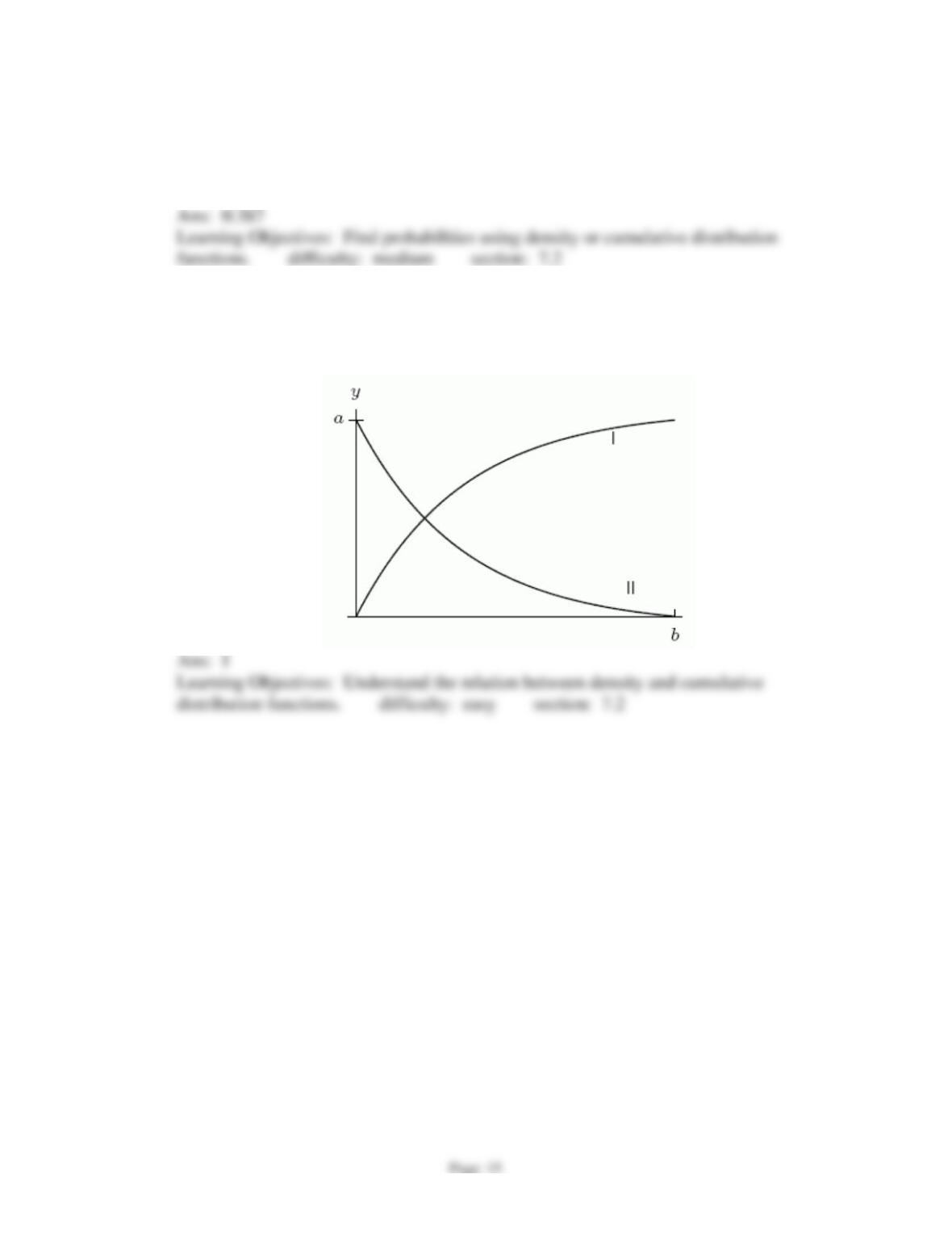
24 months
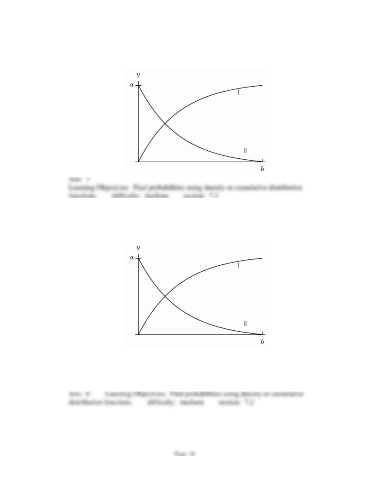
section: 7.1
4.
A density function for the lifetime of a certain type of frog is shown in the following
figure. Which is the frog’s lifetime more likely to be between?
A)
7 and 8 months
B)
10 and 11 months
C)
13 and 14 months
section: 7.1
Chapter 7
5.
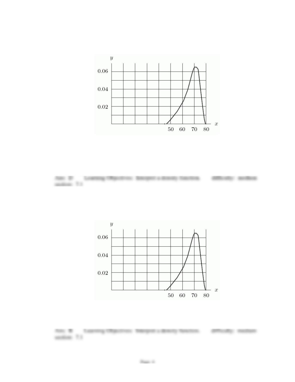
The following figure gives the density function for the number of hours students spent
studying for a calculus exam. What is the largest amount of time a student spent
studying?
A)
1 hour
B)
3 hours
C)
4 hours
D)
6 hours
E)
8 hours
section: 7.1
6.
The following figure gives the density function for the number of hours students spent
studying for a calculus exam. Did a greater number of students study more than 2 hours
or less than 2 hours? Answer “more” or “less”.
Ans:
more
section: 7.1
Chapter 7
7.
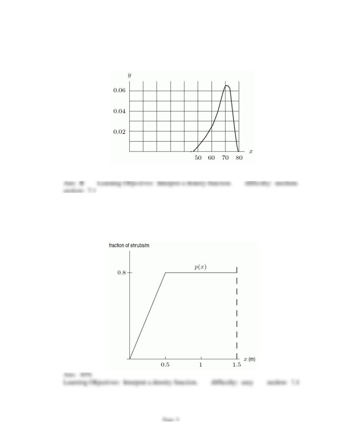
The following figure gives the density function for the velocities of cars passing a
checkpoint on a freeway. What is the most common speed?
A)
60 mph
B)
64 mph
C)
68 mph
D)
72 mph
E)
76 mph
F)
80 mph
section: 7.1
8.
The following figure gives the density function for the velocities of cars passing a
checkpoint on a freeway. What percent of the cars drove less than 60 mph?
A)
5%
B)
15%
C)
25%
D)
35%
Chapter 7
9.
The following figure gives the density function for the velocities of cars passing a
checkpoint on a freeway.Which were cars more likely to be driving?
A)
Between 55 and 65 mph
B)
Between 70 and 80 mph
section: 7.1
10.
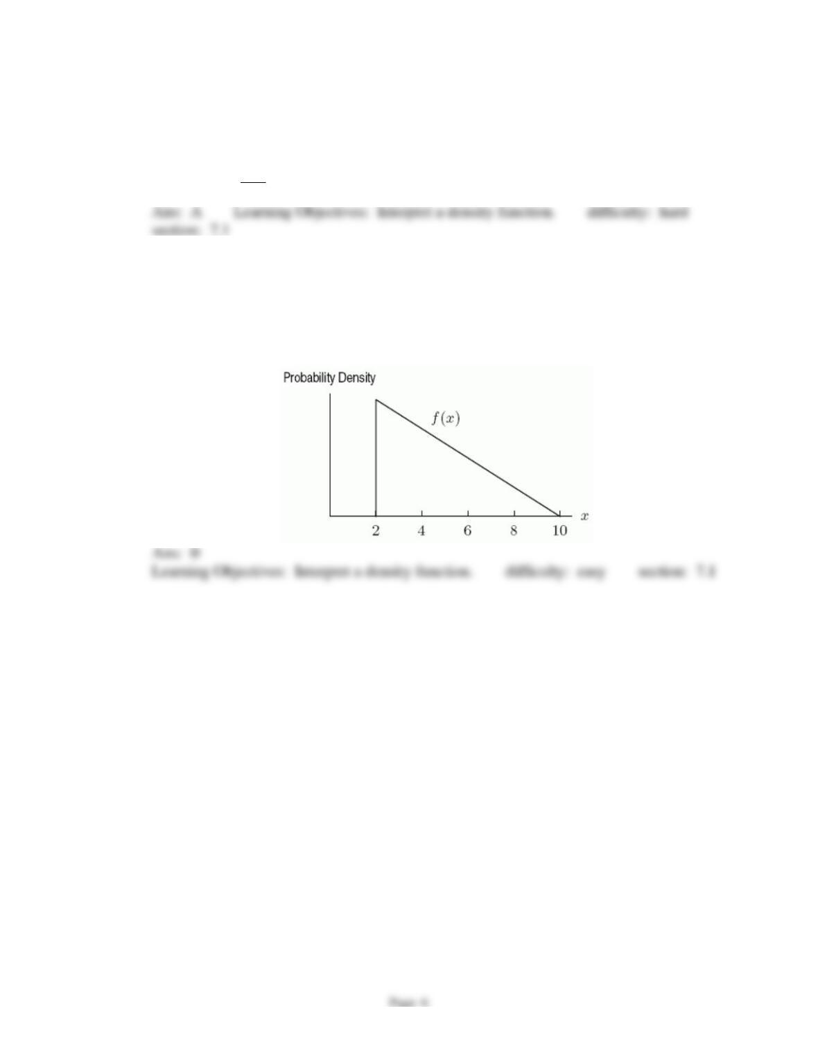
The distribution of heights, x, in meters, of a group of shrubs is represented by the
density function
()px
(no shrubs are higher than 1.5 meters). Calculate the percentage
of shrubs which are between 1 and 1.5 meter(s) high.
Ans:
40%
Learning Objectives: Interpret a density function. difficulty: easy section: 7.1
Chapter 7
11.
Which of the following could possibly be density functions? Select all that apply.
A)
( ) 0.1px =
for
15 25x
B)
( ) sinp x x=
for
03π / 2x
C)
2
() 500
x
px =
for
0 500x
12.
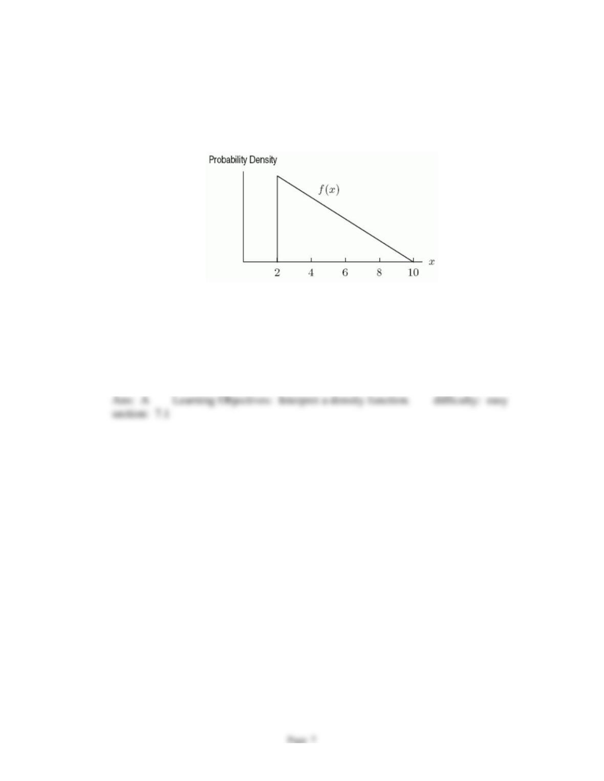
The density function f(x) shown below describes the probability that a computer circuit
board will cost a manufacturer more than a certain number of dollars to produce. In this
case, the cost of the circuit board, x, is measured in thousands of dollars. What is the
probability that the circuit board will cost less than $2 thousand to produce?
Ans:
0
Chapter 7
13.
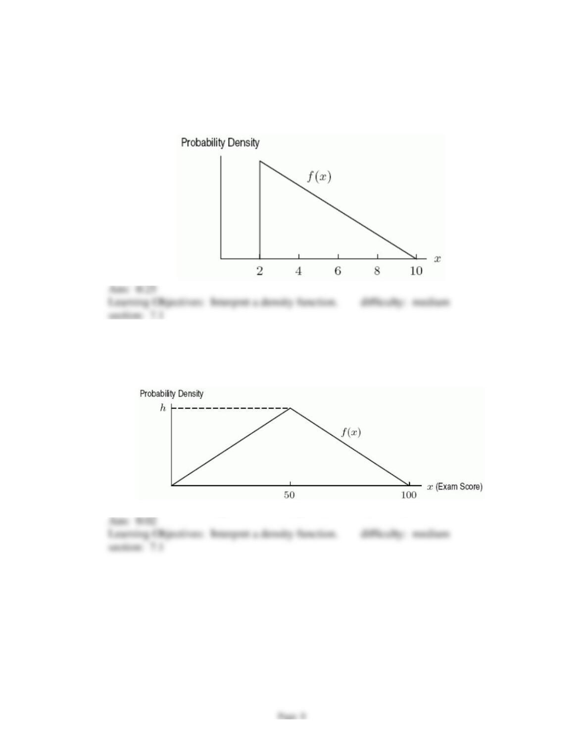
The density function f(x) shown below describes the probability that a computer circuit
board will cost a manufacturer more than a certain number of dollars to produce. In this
case, the cost of the circuit board, x, is measured in thousands of dollars. Which of the
following definite integrals give the probability that the circuit board will cost between
$2 thousand and some amount $b thousand? Assume that b is between 2 and 10.
A)
2()
bf x dx
B)
2(1 ( ))
bf x dx−
C)
10 ()
bf x dx
D)
10 (1 ( ))
bf x dx−
Chapter 7
14.
The density function f(x) shown below describes the probability that a computer circuit
board will cost a manufacturer more than a certain number of dollars to produce. In this
case, the cost of the circuit board, x, is measured in thousands of dollars. Find the
height of the triangle that describes the probability density function.
15.
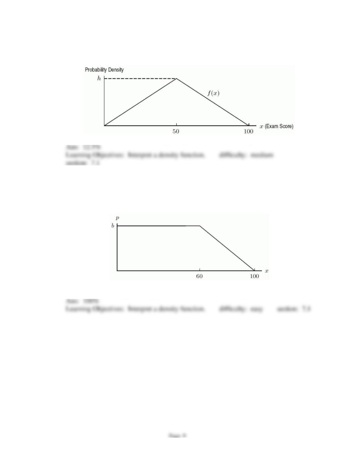
A professor far away from here gives the same 100-point final exam year after year and
discovers that the students’ scores tend to follow the triangular probability density
function f(x) pictured below:
Find the value of the height h of the triangular probability density function.
Chapter 7
16.
A professor far away from here gives the same 100-point final exam year after year and
discovers that the students’ scores tend to follow the triangular probability density
function f(x) pictured below:
What percent of the students would you expect to score below 25 points on the exam?
17.
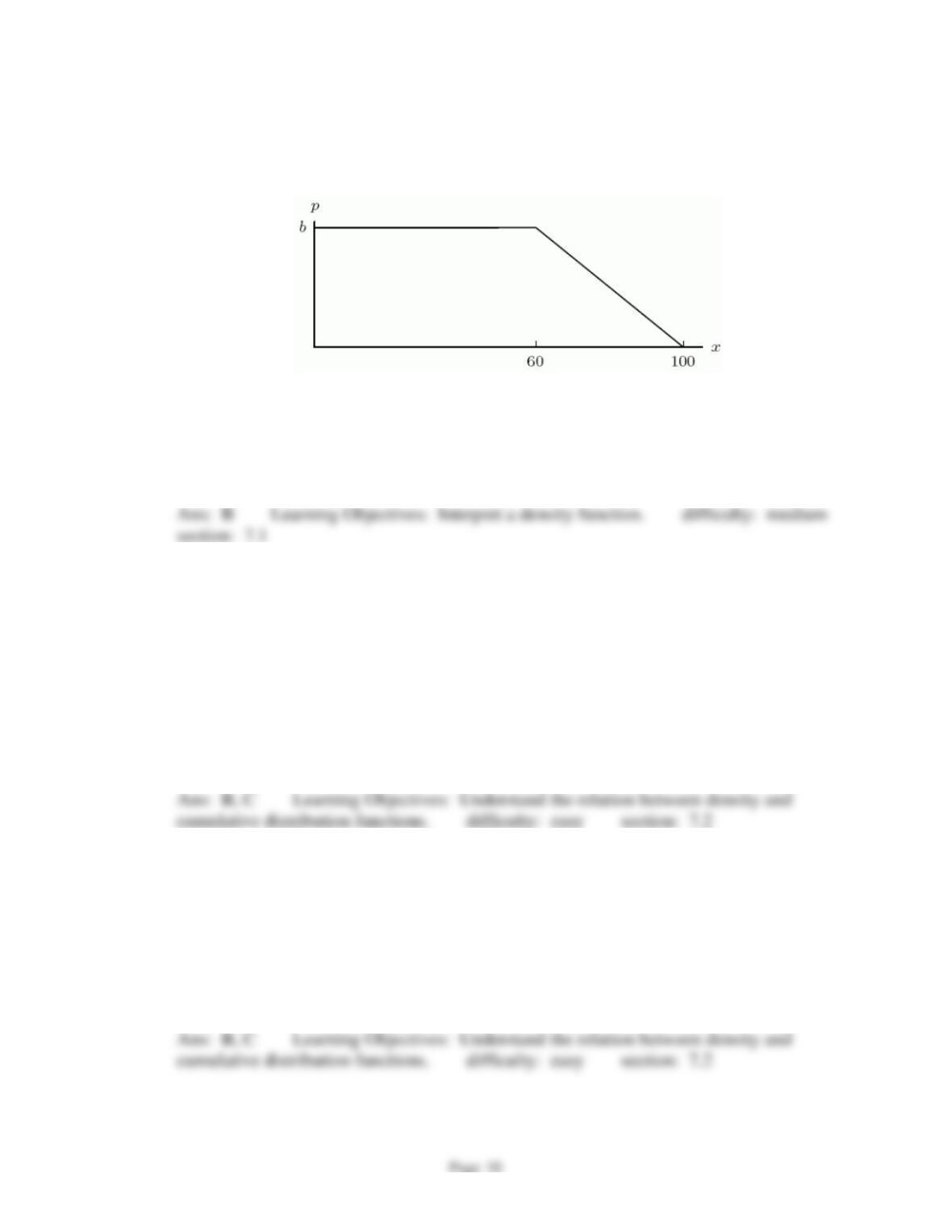
Suppose that the distribution of people’s ages in the United States is essentially constant,
or uniform, from age 0 to age 60, and from there it decreases linearly until age 100. This
distribution p(x) is shown below, where x is age in years, and p measures probability
density. Such a probability distribution is called trapezoidal.
According to this simplified model of the distribution of people’s ages in the United
States, what percentage of the population is between 0 and 100 years old?
Chapter 7
18.
Suppose that the distribution of people’s ages in the United States is essentially constant,
or uniform, from age 0 to age 60, and from there it decreases linearly until age 100. This
distribution p(x) is shown below, where x is age in years, and p measures probability
density. Such a probability distribution is called trapezoidal.
In terms of b (see the graph), find the fraction of the population that is between 60 and
100 years old.
A)
60b
B)
20b
C)
40b
D)
80b
19.
Suppose
()px
is a density function for a certain distribution and
()Px
is the
cumulative distribution function for the same distribution. Which of the following
gives the fraction of the distribution between x = 7 and x = 16? Select all that apply.
A)
16
7()P x dx
B)
16
7()p x dx
C)
(16) (7)PP−
D)
(16) (7)pp−
20.
Suppose
()Px
is the cumulative distribution function for sizes of graduating classes
among a group of high schools and
(150) 0.4P=
. Which of the following are possible
statements about
(175)P
?
A)
(175) 0.4P
B)
(175) 0.4P=
C)
(175) 0.4P
Chapter 7
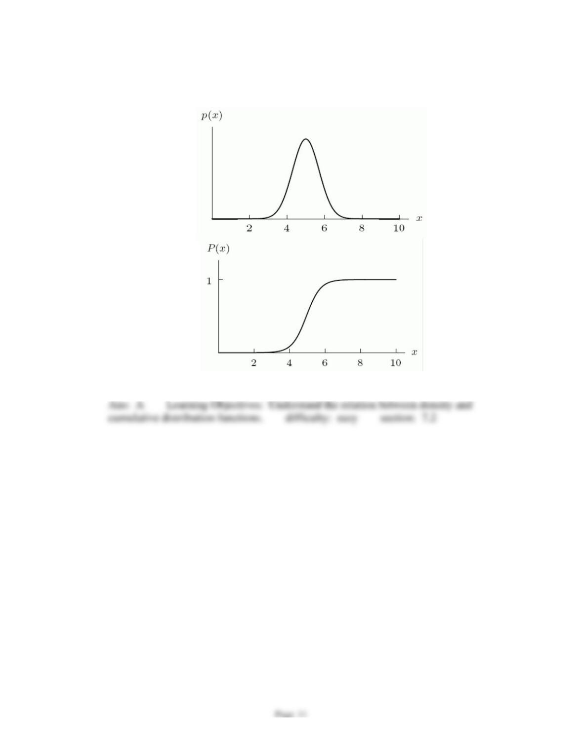
21.
The cumulative distribution function in the second graph corresponds to the density
function in the first graph.
A)
True
B)
False
cumulative distribution functions. difficulty: easy section: 7.2
Chapter 7
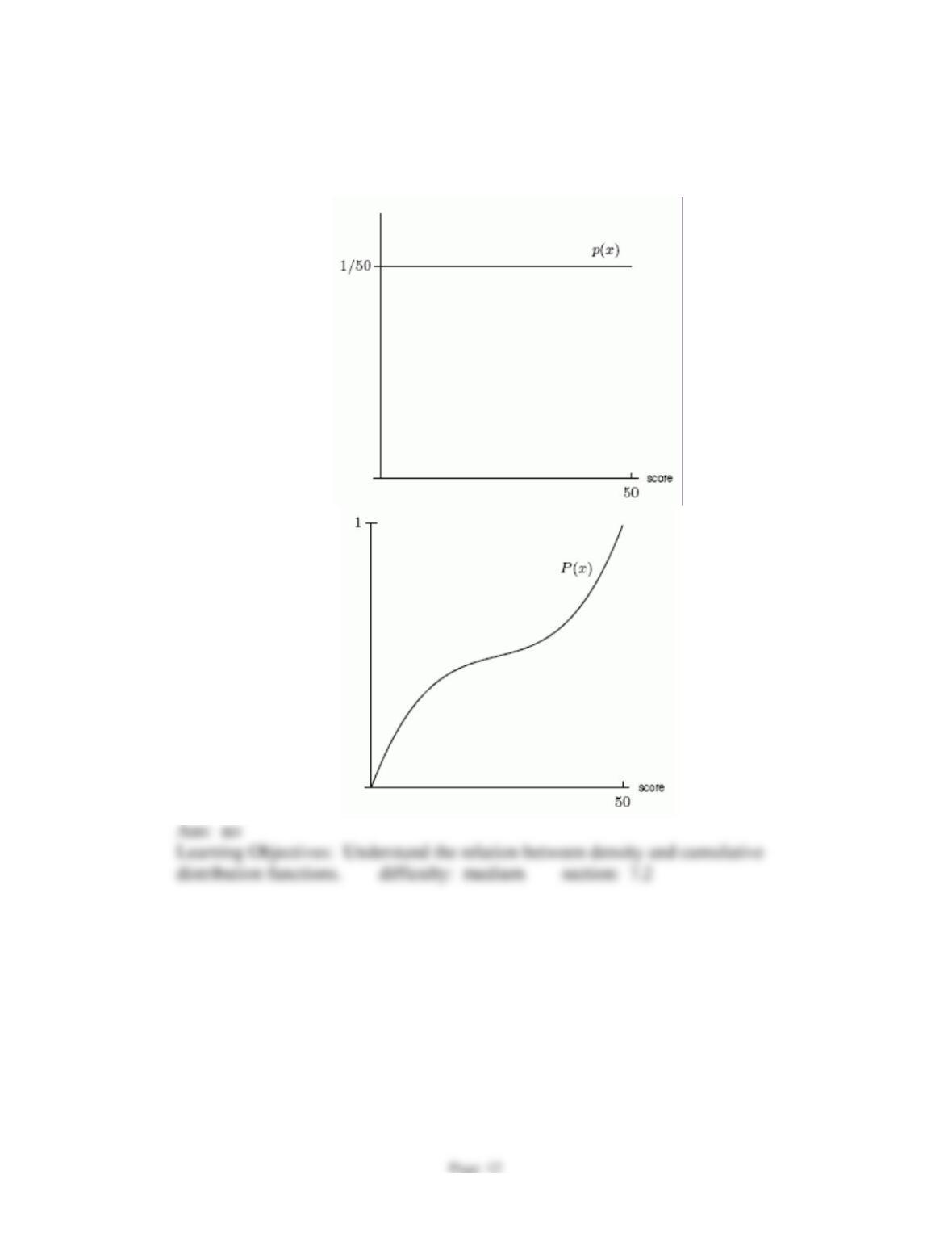
22.
An aptitude test is given to a group of students. Scores can range from 0 to 50. Does
the cumulative distribution function in the second graph correspond to the density
function in the first graph? Answer “yes” or “no”
Chapter 7
23.
The cumulative distribution function for the time to complete a step on an assembly line
is given in the following table. What percent of the steps take from 0 to 14 minutes to
complete?
t min
6
8
10
12
14
16
18
20
()Pt
0
0.03
0.15
0.21
0.54
0.78
0.86
0.97
Chapter 7
Page 14
24.
Which of the following cumulative distribution graphs would most likely represent the
total annual sales of milk?
I. II.
III.
25.
The density function for the height of trees in a forest is given by
5
( ) 0.000006p x x=
,
where x is height in meters and the tallest tree is 10 meters. Find the cumulative
distribution function,
()Px
, for this density function.
Chapter 7
26.
The density function for the height of trees in a forest is given by
2
( ) 0.003p x x=
,
where x is height in meters and the tallest tree is 10 meters. Find the probability, to 3
decimal places, that a tree is between 5 and 8 meters tall.
Ans:
0.387
Learning Objectives: Find probabilities using density or cumulative distribution
functions. difficulty: medium section: 7.2
27.
The following figure shows a density function and the corresponding distribution
function. Which curve represents the cumulative distribution function?
Ans:
I
Learning Objectives: Understand the relation between density and cumulative
distribution functions. difficulty: easy section: 7.2
Chapter 7
28.
The following figure shows a density function and the corresponding distribution
function. What is the value of a?
Ans:
1
functions. difficulty: medium section: 7.2
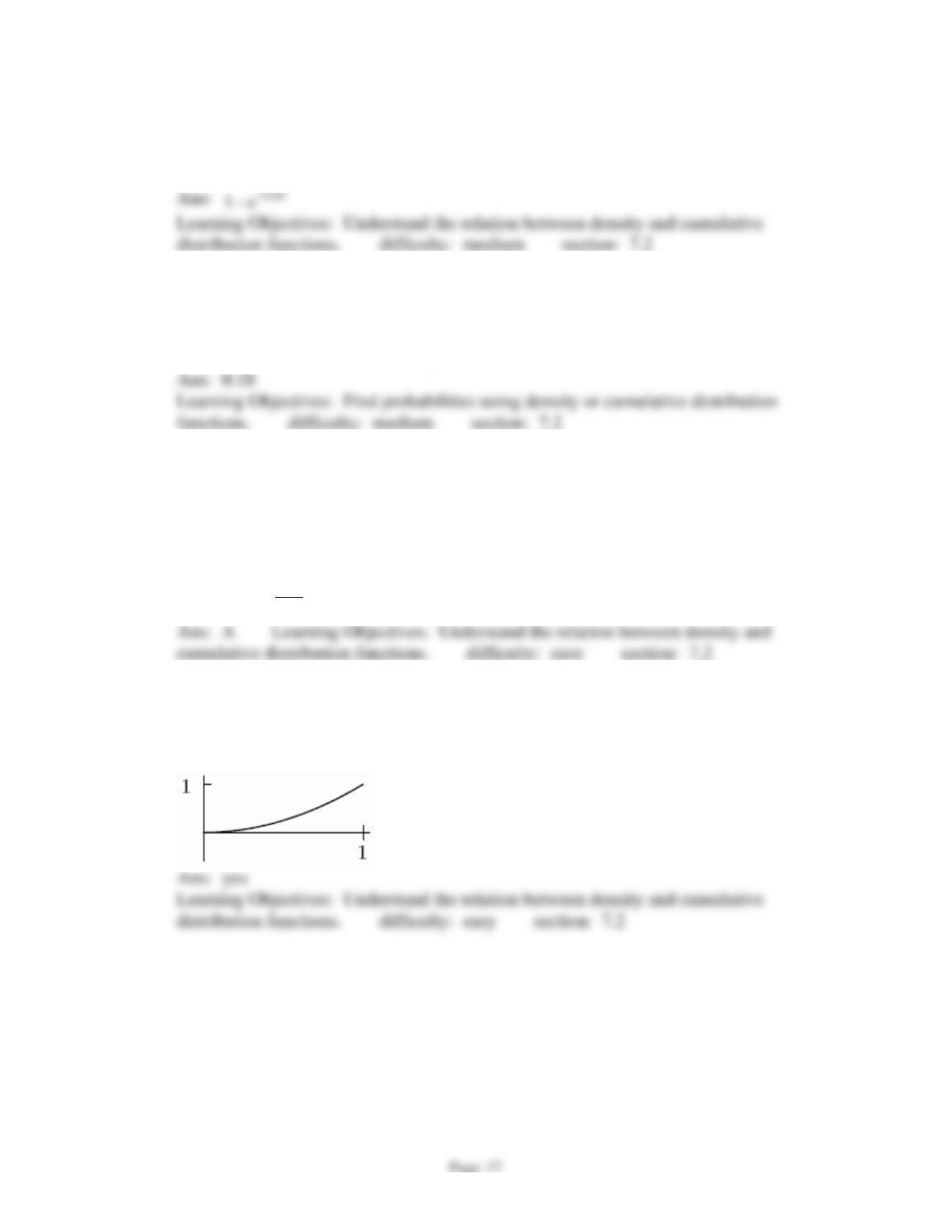
29.
The following figure shows a density function and the corresponding distribution
function. The drawing is not to scale. What is a reasonable estimate for b?
A)
1
B)
2
C)
3
D)
4
E)
cannot be determined
distribution functions. difficulty: medium section: 7.2
Chapter 7
30.
The life expectancy of a bug can be approximated by the density function
0.25
( ) 0.25 t
p t e−
=
, where t is time in days. Find the cumulative distribution function,
()Pt
, associated with this density function.
Learning Objectives: Understand the relation between density and cumulative
distribution functions. difficulty: medium section: 7.2
31.
The life expectancy of a bug can be approximated by the density function
0.3
( ) 0.3 t
p t e−
=
, where t is time in days. Find the probability that a bug lives between 3
and 5 days. Round to 2 decimal places.
Ans:
0.18
Learning Objectives: Find probabilities using density or cumulative distribution
functions. difficulty: medium section: 7.2
32.
Which of the following could possibly be cumulative distribution functions? Select all
that apply.
A)
( ) 0.1 1P x t=−
for
30 40t
B)
( ) 1 cosP x x=−
for
03π / 2x
C)
3
() 100
x
Pt =
for
0 100x
33.
Let p(t) be a probability density which is defined for 0 t 1. Could the following be
the cumulative distribution function for p?
Ans:
yes