Chapter 5 – Network Models
1. Problems which deal with the direct distribution of products from supply locations to demand locations are called:
a.
transportation problems
b.
assignment problems
c.
network problems
d.
transshipment problems
a
1
2. The objective in transportation problems is typically to:
a.
maximize profits
b.
maximize revenue
c.
minimize costs
d.
maximize feasibility
c
1
3. A particularly useful Excel function in the formulation of transportation problems is the:
a.
IF function
b.
SUMIF function
c.
SUMPRODUCT function
d.
NPV function
c
1
4. The decision variables in transportation problems are:
a.
profits
b.
costs
c.
flows
d.
capacities
c
1
5. For all routes with positive flows in an optimized transportation problem, the reduced cost will be:
a.
zero
b.
how much less shipping costs would have to be for shipments to occur along that route
c.
how much more shipping costs would have to be for shipments to occur along that route
d.
how much the capacity is along that shipping route
a
1
6. The network model representation of the transportation problem has the following advantage relative to the special case
of a simple transportation model:
a.
it does not require capacity restrictions on the arcs of the network
b.
the flows in the network model don’t all necessarily have to be from supply locations to demand locations
c.
a network model representation is generally easier to formulate and solve
Chapter 5 – Network Models
d.
All of these options
b
1
7. In a typical network model representation of the transportation problem, the nodes indicate
a.
roads
b.
rail lines
c.
geographic locations
d.
rivers
c
1
8. In a minimum cost network flow model, the flow balance constraint for each supply node has the form
a.
Flow in ≥ Flow out + Net supply
b.
Flow out ≥ Flow in + Net demand
c.
Flow in = Flow out
d.
Flow out ≤ Flow in + Net supply
e.
Flow in ≤ Flow out + Net demand
d
1
9. In an assignment model of machines to jobs, the machines are analogous to which of the following in a transportation
problem?
a.
Suppliers
b.
Customers
c.
Flows
d.
Unit capacities
a
1
10. Which of the following is not an example of a condition that a more complex logistics model might include?
a.
Multiple products
b.
Multiple modes of transportation
c.
Multiple time periods
d.
Multiple objectives
d
1
11. The graphical representation of a network in an optimization problem can be an aid in the development of a
spreadsheet model.
a.
True
b.
False
1
12. It is useful to model network problems by listing all of the arcs and their corresponding flows in one long,
comprehensive list.
a.
True
b.
False
True
1
13. In transportation problems, shipments between supply points or between demand points are possible.
a.
True
b.
False
False
1
14. In transportation problems, the three sets of input numbers that are required are capacities, demands and flows.
a.
True
b.
False
False
1
15. In network models of transportation problems, arcs represent the routes for getting a product from one node to
another.
a.
True
b.
False
True
1
16. In an optimized shipping plan, most of the shipments occur on the low-cost routes, but this is not always the case.
a.
True
b.
False
True
1
17. Transshipment points are locations where goods neither originate nor end up, but goods are allowed to enter such
points to be shipped out to their eventual destinations.
a.
True
b.
False
True
1
18. The flow balance constraint for each transshipment node in a network flow model has the form Flow in = Flow out.
a.
True
b.
False
True
1
19. A typical shortest path problem is a special case of the general network flow model.
Chapter 5 – Network Models
a.
True
b.
False
True
1
20. The cost of an arc in a shortest path problem is equal to the distance of the arc.
a.
True
b.
False
False
1
Exhibit 5-1
Sinclair Plastics operates two chemical plants which produce polyethylene; the Ohio Valley plant which can produce up to
10,000 tons per month and the Lakeview plant which can produce up to 7,000 tons per month. Sinclair sells its
polyethylene to three different auto manufacturing plants, Grand Rapids (demand = 3000 tons per month), Blue Ridge
(demand = 5000 tons per month), and Sunset (demand = 4000 tons per month). The costs of shipping between the
respective plants is shown in the table below:
Grand Rapids
Blue Ridge
Sunset
Ohio Valley
50
40
100
Lakeview
60
50
75
21. Refer to Exhibit 5-1. Formulate (write out algebraically) an LP transportation model to help Sinclair minimize its
shipping costs.
1
22. Refer to Exhibit 5-1. Implement the LP model in Solver and obtain the optimal shipping plan. What is the optimized
cost?
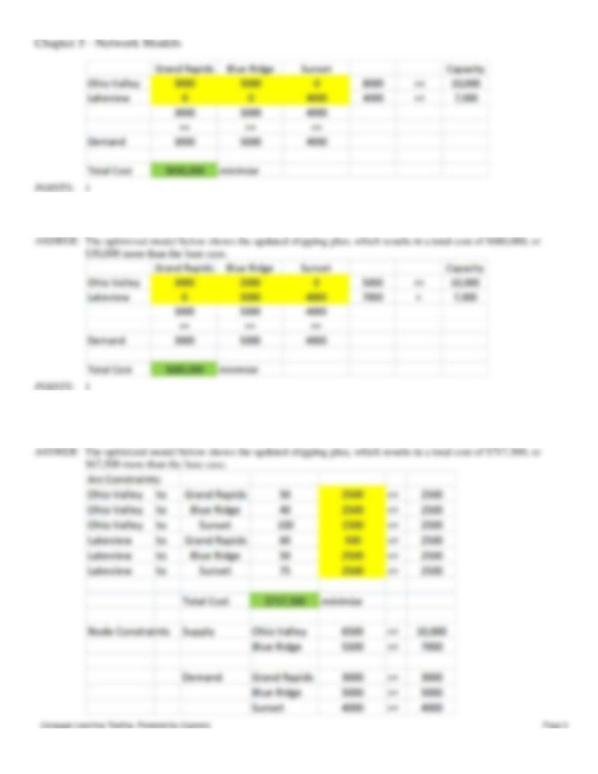
23. Refer to Exhibit 5-1. Suppose the Lakeview plant was required to run at capacity. How much more would the shipping
plan cost Sinclair?
24. Refer to Exhibit 5-1. Suppose the shipping capacity between any two plants was limited to 2500 tons per month.
Design and implement a network flow version of this model in Solver and obtain the optimal shipping plan. How much
more would the shipping plan cost Sinclair in that case?
Chapter 5 – Network Models
Exhibit 5-2
A small engineering firm employs one civil engineer, two engineering technicians, and one summer intern. The types of
projects the firm does includes surveys (typically 7 per month), designs (5 per month), and construction project plans
(four per month). The times, in hours, required for each employee to complete teach type of project are shown below.
Based on their capabilities and time spent on travel and administrative tasks, the engineer, tech 1, tech 2, and intern can
handle 5, 4, 4, and 3 projects per month, respectively.
Survey
Design
Plan
Engineer
30
35
30
Technician 1
25
50
45
Technician 2
20
55
40
Intern
35
45
55
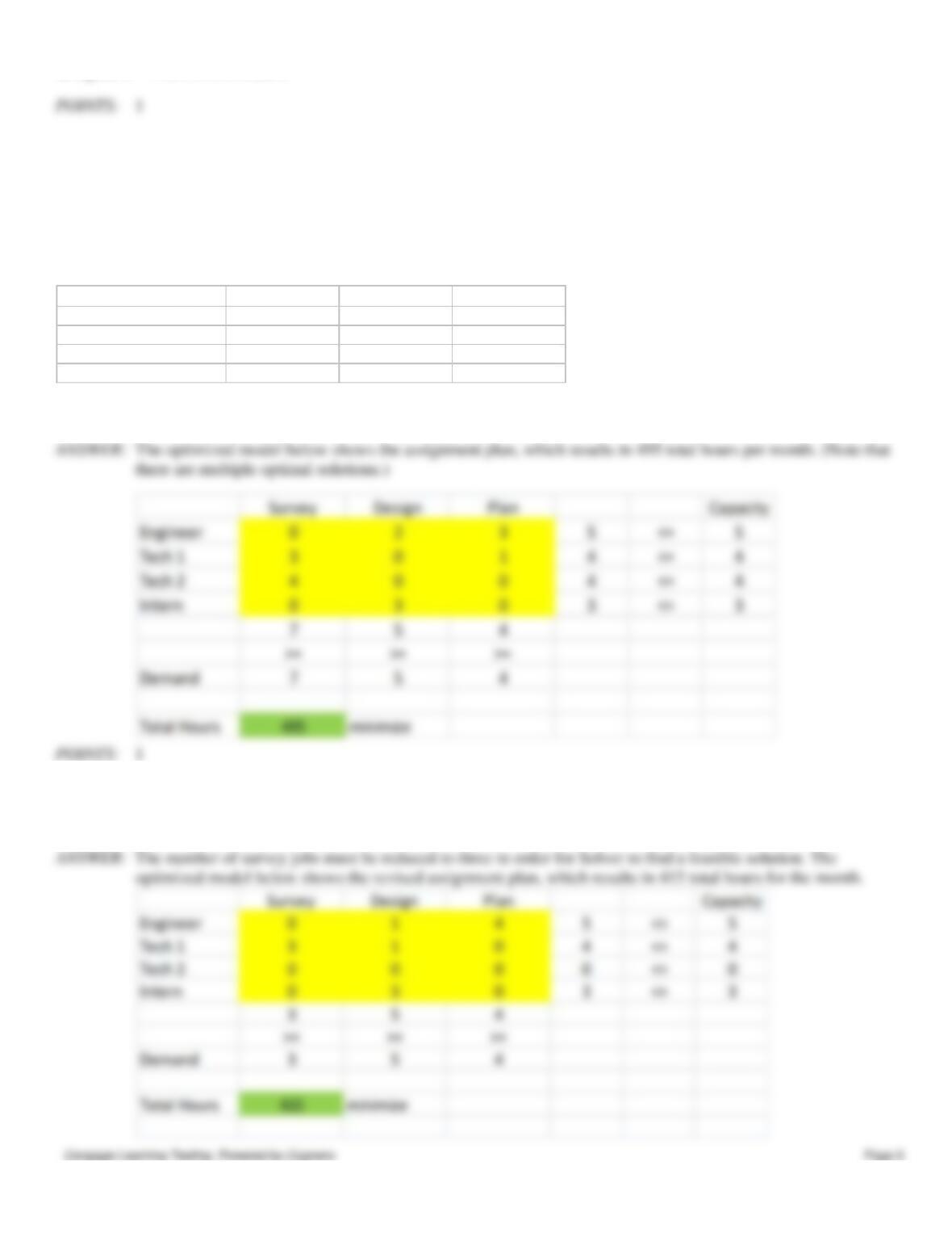
25. Refer to Exhibit 5-2. Implement a LP model in Solver and determine the optimal monthly assignment plan for the
firm. What is the total number of hours that will be assigned to projects each month?
26. Refer to Exhibit 5-2. Suppose Tech 2 will not be available during the next month. Keeping the same number of design
and construction plan projects, how many survey projects would the firm be able to do? What would be the revised
assignment plan in that case?
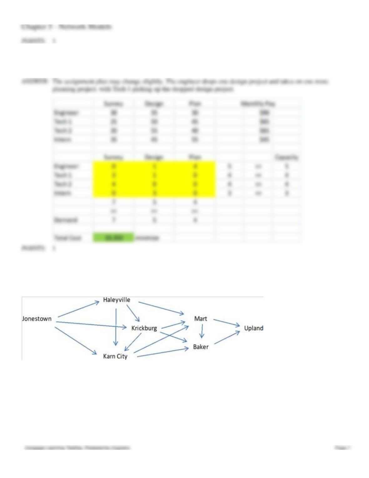
27. Refer to Exhibit 5-2. Based on their salaries, the engineer, tech 1, tech 2, and intern earn $90, $65, $65, and $45 per
hourly, respectively. Change the firm’s objective function to minimize staff costs and find the optimal assignment plan.
Does it change from the base case?
Exhibit 5-3
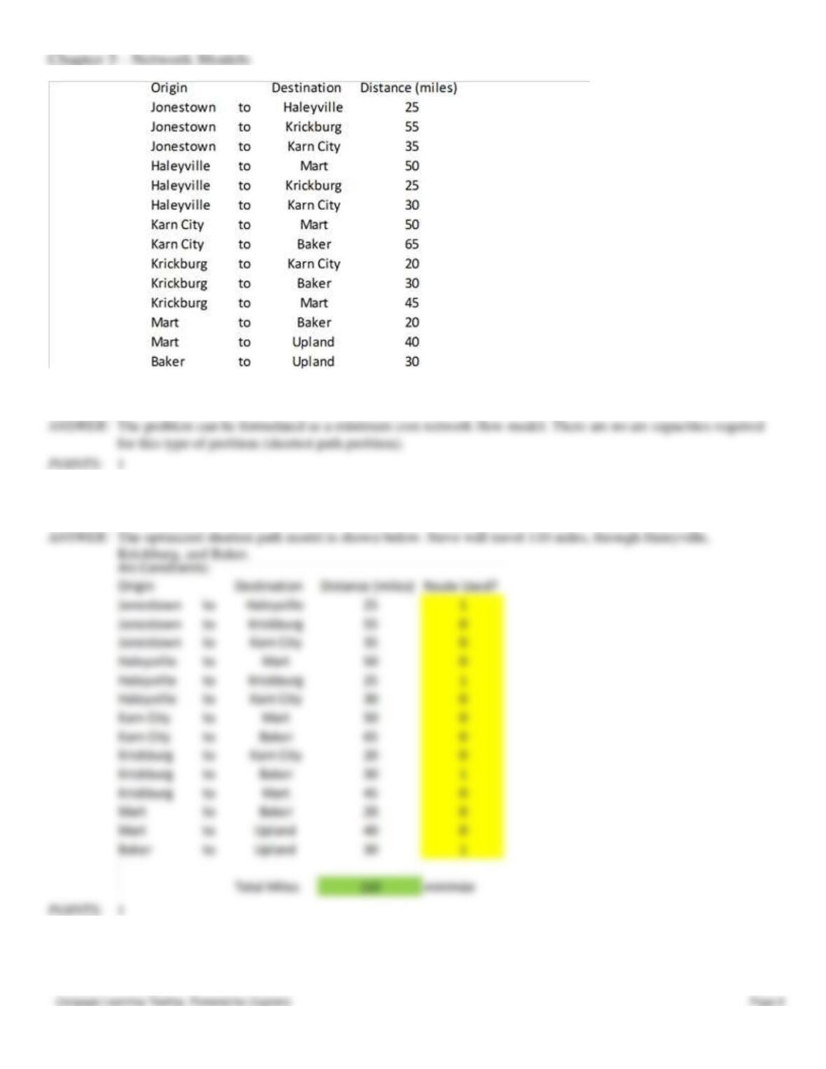
Steve the auto parts salesman is trying to navigate his way between the rural west Texas towns of Jonestown and Upland.
The possible routes for this trip are shown below, along with the mileage along each route.
28. Refer to Exhibit 5-3. What general type of LP model can be applied to this problem? What modifications to the
general type are required for this problem?
The problem can be formulated as a minimum cost network flow model. There are no arc capacities required
for this type of problem (shortest path problem).
29. Refer to Exhibit 5-3. Implement the appropriate model in Solver and determine the shortest path for Steve. How many
total miles will he travel on his trip?
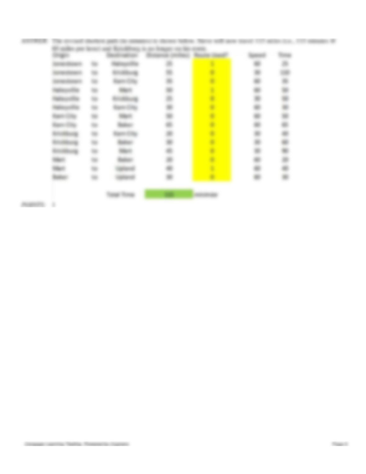
30. Refer to Exhibit 5-3. Suppose the roads leading into and out of Krickburg are unpaved, so Steve would only be able to
travel half of his usual 60 mile/hour speed on those routes. Modify the model to account for this condition. Would the
shortest path change from the base case solution?
Chapter 5 – Network Models