38) Production data for the number of hours required per unit for making the Droid and iPhone
versions of cell phone components by Bizzer, a high-tech manufacturing firm, is given below.
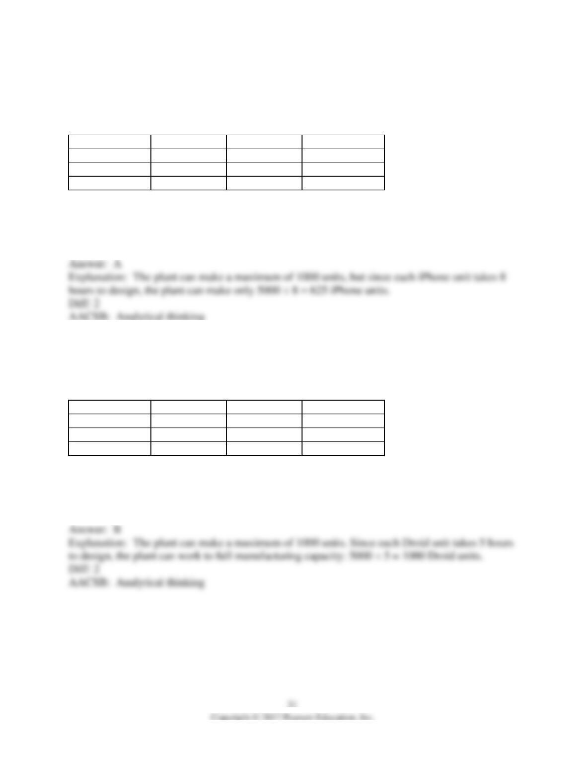
What is the maximum number of iPhone units that the factory can make?
Monthly Product
Droid iPhone Capacity (Hours)
Design 5 8 5000
Manufacture 2.5 2.5 2500
Profit per unit $4 $6
A) 625
B) 1000
C) 5000
D) 800
39) Production data for the number of hours required per unit for making the Droid and iPhone
versions of cell phone components by Bizzer, a high-tech manufacturing firm, is given below.
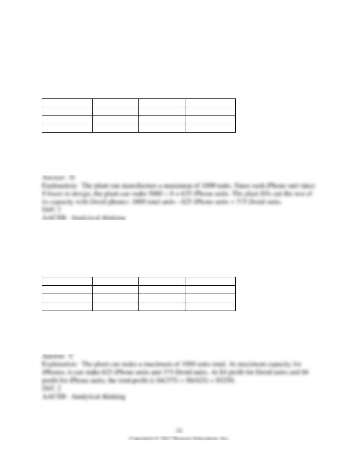
What is the maximum number of Droid units that the factory can make?
Monthly Product
Droid iPhone Capacity (Hours)
Design 5 8 5000
Manufacture 2.5 2.5 2500
Profit per unit $4 $6
A) 625
B) 1000
C) 5000
D) 800
40) Production data for the number of hours required per unit for making the Droid and iPhone
versions of cell phone components by Bizzer, a high-tech manufacturing firm, is given below.
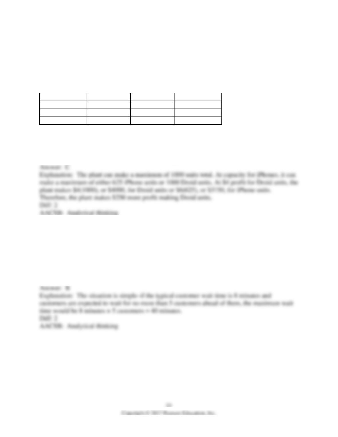
Suppose the plant decides to make the maximum number of iPhone components possible and
reach the rest of its capacity by making Droid phones. How many of each type of phone will it
make?
Monthly Product
Droid iPhone Capacity (Hours)
Design 5 8 5000
Manufacture 2.5 2.5 2500
Profit per unit $4 $6
A) 375 iPhone units and 625 Droid units
B) 500 iPhone units and 500 Droid units
C) 1000 iPhone units and 1000 Droid units
D) 625 iPhone units and 375 Droid units
41) Production data for the number of hours required per unit for making the Droid and iPhone
versions of cell phone components by Bizzer, a high-tech manufacturing firm, is given below.
Suppose the plant decides to make the maximum number of iPhone components possible and
reach the rest of its capacity by making Droid phones. How much profit will it make?
Monthly Product
Droid iPhone Capacity (Hours)
Design 5 8 5000
Manufacture 2.5 2.5 2500
Profit per unit $4 $6
A) $3750
B) $1500
C) $5250
D) $4000
42) Production data for the number of hours required per unit for making the Droid and iPhone
versions of cell phone components by Bizzer, a high-tech manufacturing firm, is given below.
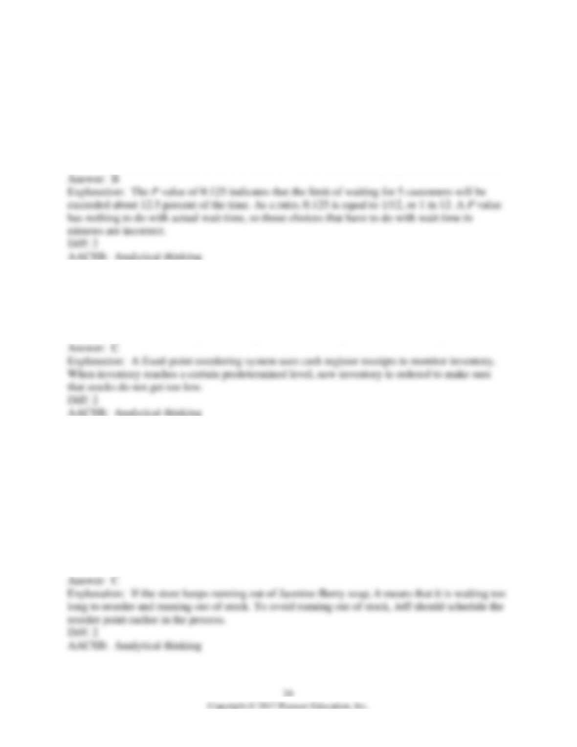
Suppose the plant decides exclusively to make either the maximum number of iPhone
components or the maximum number of Droid phones. Which choice will result in the greater
profit?
Monthly Product
Droid iPhone Capacity (Hours)
Design 5 8 5000
Manufacture 2.5 2.5 2500
Profit per unit $4 $6
A) Making Droid units will result in $4000 more profit.
B) Making iPhone units will result in $250 more profit.
C) Making Droid units will result in $250 more profit.
D) Making iPhone units will result in $3750 more profit.
43) A queuing theory analysis for the Department of Motor Vehicles determines that customers
typically wait for 8 minutes and that the agency should strive never to exceed more than 5
customers in a single line. What is the maximum amount of time that customers should be
expected to wait?
A) 8 minutes
B) 40 minutes
C) 20 minutes
D) 24 minutes
44) A queuing theory analysis for the Department of Motor Vehicles determines that customers
typically wait for 8 minutes and that the agency should strive never to exceed more than 5
customers in a single line. An analysis comes up with a value for P of 0.125. What does this P
value mean?
A) that customers will wait an average of 12.5 minutes
B) that the chances that a customer will need to wait for more than 5 people in line are 1 in 8
C) that customers will wait an average of 0.125 minutes
D) that the chances that a customer will need to wait for more than 5 people in line are 1 in 12.5
45) How does a fixed-point reordering system work?
A) When inventory level reaches 50 percent of maximum, the system orders new inventory.
B) When inventory level reaches 33 percent of maximum, the system orders new inventory.
C) At some preestablished inventory level, the system automatically orders new inventory.
D) At some random inventory level, the system automatically orders new inventory.
46) Jeff, a manager at the Flux Soap Store, notices that the store regularly runs out of Jasmine-
Berry soap. Currently, the reorder point is fixed when inventory reaches 40 percent of maximum.
Which adjustment should Jeff make in a fixed-point reordering system?
A) Jeff should lower the reorder level to a point where inventory of Jasmine-Berry soap is at 30
percent of maximum.
B) Jeff should lower the reorder level to a point where inventory of Jasmine-Berry soap is at 10
percent of maximum.
C) Jeff should raise the reorder level to a point where inventory of Jasmine-Berry soap is at 50
percent of maximum.
D) Jeff should lower the reorder level to a point where inventory of Jasmine-Berry soap is at half
of the previous level.
47) Jeff, a manager at the Flux Soap Store, lowered the reorder point for Butterscotch-Lemon
soap from 33 percent of maximum to 20 percent of maximum. What is Jeff likely to observe?
A) The level of Butterscotch-Lemon soap in stock should increase.
B) Sales of Butterscotch-Lemon soap should decrease.
C) Sales of Butterscotch-Lemon soap should increase.
D) The level of Butterscotch-Lemon soap in stock should drop.
48) Which of the following identifies the goal of managers who use the economic order quantity
(EOQ) model?
A) minimizing carrying costs and ordering costs
B) maximizing carrying costs and ordering costs
C) maximizing carrying costs and minimizing ordering costs
D) maximizing carrying costs and total costs
49) Mia, a manager at Best Buy, increases the order size for a product that the company sells,
which will ________.
A) increase both ordering costs and carrying costs
B) increase ordering costs and decrease carrying costs
C) decrease both ordering costs and carrying costs
D) decrease ordering costs and increase carrying costs
50) Mia, a manager at Best Buy, should be able to find Q, the most economic order size for a
product, by ________.
A) locating where the carrying costs curve and the total costs curve intersect
B) locating where the carrying costs curve and the ordering costs curve intersect
C) locating where the carrying costs curve and the ordering costs curve are parallel
D) locating where the total costs curve and the ordering costs curve are parallel
51) A new upgrade for a product is expected to increase demand by a factor of 4. If all other
factors remain equal, how is EOQ likely to change?
A) EOQ will double.
B) EOQ will increase by 50 percent.
C) EOQ will decrease by 50 percent.
D) EOQ will not change.
52) An optimistic manager will typically follow a maximax choice.
53) A pessimistic manager will typically follow a minimin choice.
54) With choice S1, a manager sees gains of $10 million and $6 million. With choice S2, a
manager sees gains of $12 million and $3 million. The manager chooses S2, so she must be
optimistic.
55) With choice S1, a manager sees gains of $10 million and $6 million. With choice S2, a
manager sees gains of $12 million and $8 million. S2 might be the choice of a pessimistic
manager.
56) With choice S1, a manager sees gains of $10 million and $6 million. With choice S2, a
manager sees gains of $12 million and $8 million. Only a pessimistic manager would choose S1.
57) Regret is computed by subtracting the value of a possible strategy from the greatest value in
the entire matrix.
58) This payoff matrix gives values for strategies S1, S2, and S3 for the Bigg Company and
competitive strategies CA1, CA2, and CA3 for the Large Company. From Bigg’s point of view,
the S1 maximum regret for CA1 is 8.
CA1 CA2 CA3
S1 8 5 12
S2 9 14 3
S3 16 13 20
59) This payoff matrix gives values for strategies S1, S2, and S3 for the Bigg Company and
competitive strategies CA1, CA2, and CA3 for the Large Company. From Bigg’s point of view,
the S1 maximum regret for CA2 is 8.
CA1 CA2 CA3
S1 8 5 12
S2 9 14 3
S3 16 13 20
60) This payoff matrix gives values for strategies S1, S2, and S3 for the Bigg Company and
competitive strategies CA1, CA2, and CA3 for the Large Company. From Bigg’s point of view,
the S2 maximum regret is 9.
CA1 CA2 CA3
S1 8 5 12
S2 9 14 3
S3 16 13 20
61) This payoff matrix gives values for strategies S1, S2, and S3 for the Bigg Company and
competitive strategies CA1, CA2, and CA3 for the Large Company. From Bigg’s point of view,
the S3 maximum regret is 1.
CA1 CA2 CA3
S1 8 5 12
S2 9 14 3
S3 16 13 20
62) This regret matrix gives values for strategies S1, S2, and S3 for the Bigg Company and
competitive strategies CA1, CA2, and CA3 for the Large Company. A minimax Bigg manager
would choose S2 because it has the smallest maximum regret of 1.
CA1 CA2 CA3
S1 5 5 3
S2 9 6 1
S3 10 2 5
63) This regret matrix gives values for strategies S1, S2, and S3 for the Bigg Company and
competitive strategies CA1, CA2, and CA3 for the Large Company. The maximum regrets for
this table are S1 = 5, S2 = 9, S3 = 12.
CA1 CA2 CA3
S1 5 5 3
S2 9 6 1
S3 10 2 5
64) This regret matrix gives values for strategies S1, S2, and S3 for the Bigg Company and
competitive strategies CA1, CA2, and CA3 for the Large Company. A minimax Bigg manager
choosing S3 would have a greatest possible regret of 2.
CA1 CA2 CA3
S1 5 5 3
S2 9 6 1
S3 10 2 5
65) Decision trees are unreliable for making pricing decisions.
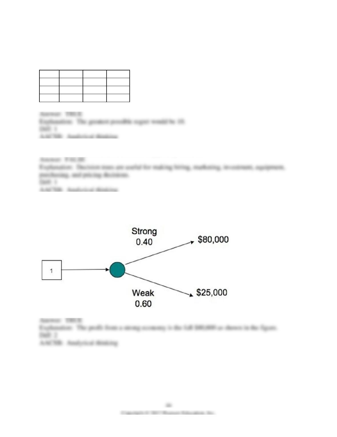
66) The decision tree shows the profit outcomes for a sandwich shop in a strong and a weak
economy. If the economy is strong, the shop is likely to make an $80,000 profit.
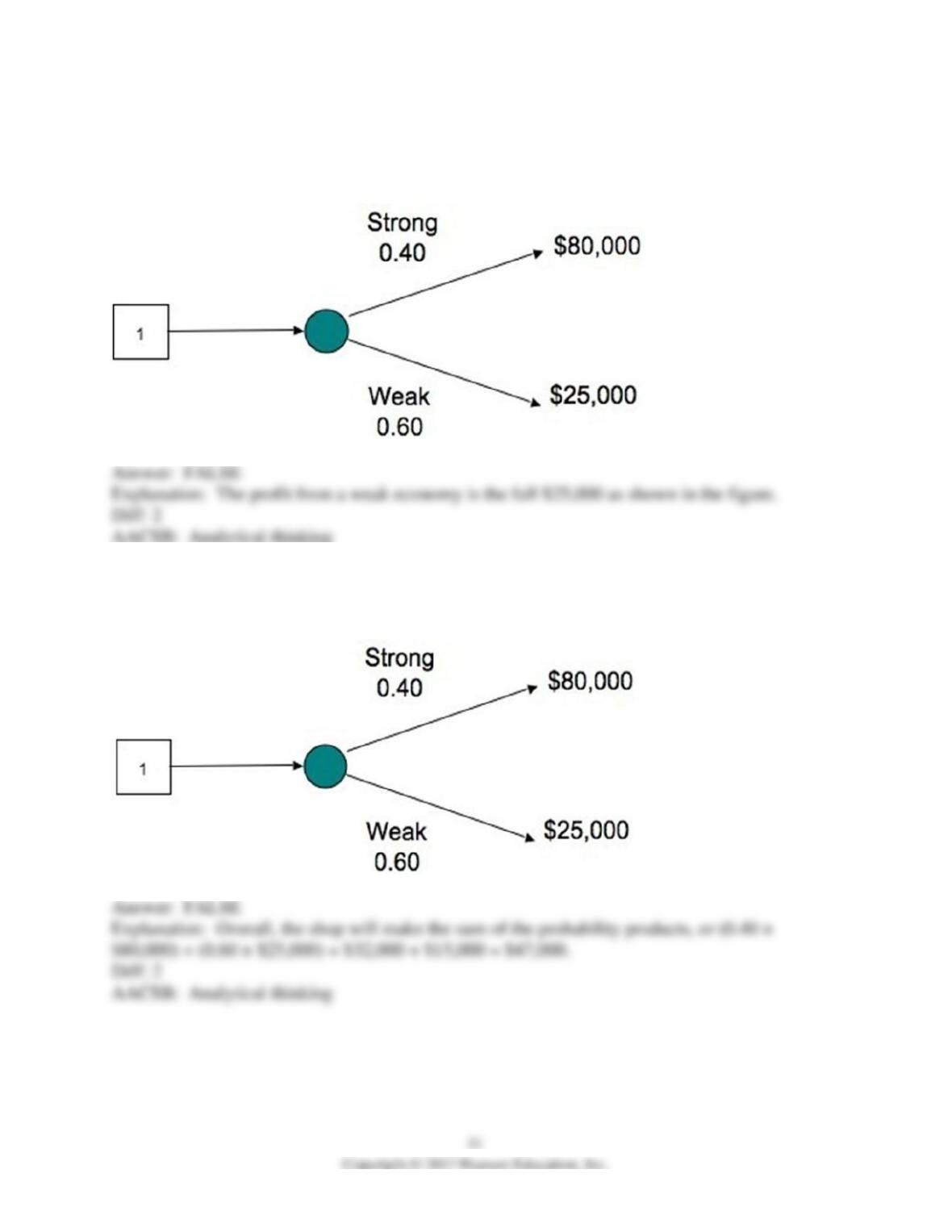
67) The decision tree shows the profit outcomes for a sandwich shop in a strong and a weak
economy. If the economy is weak, the shop is likely to make 60 percent of a $25,000 profit, or
$15,000.
68) The decision tree shows the profit outcomes for a sandwich shop in a strong and a weak
economy. Overall, the shop is expected to make $32,000.
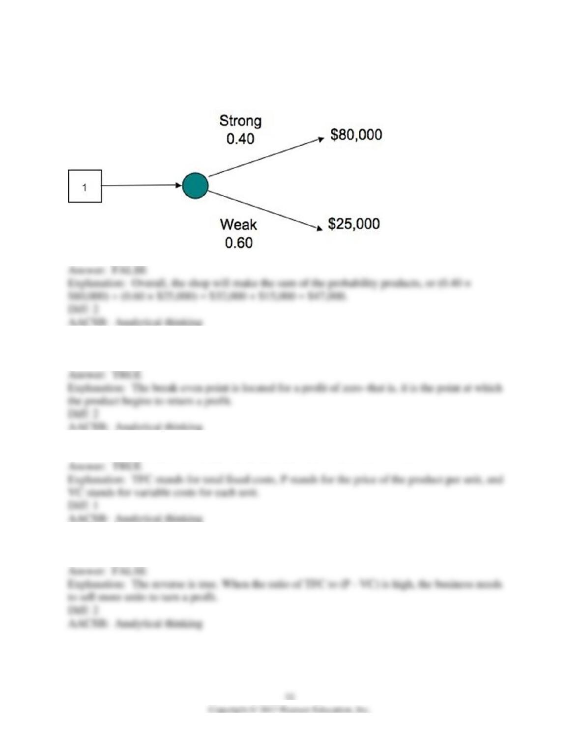
69) The decision tree shows the profit outcomes for a sandwich shop in a strong and a weak
economy. The shop is likely to make $105,000, the sum of both projections.
70) A manager uses break-even analysis to find out how many units of a product he needs to sell
to make a profit of zero.
71) The break-even point is computed by the formula BE = [TFC/(P – VC)].
72) The greater the ratio of TFC to (P – VC) is means that the business needs to sell fewer units
to make a profit.
73) Reducing the value of VC in a break-even analysis means that the business needs to sell
fewer units to turn a profit.
74) Liquidity is a measure of an organization’s ability to access cash to meet its debt obligations.
75) A current ratio of 1.5 to 1 for an organization suggests that the organization will not be able
to meet its short-term debt obligations.
76) An organization with a high leverage ratio has usually been overly cautious and conservative
in its borrowing.
77) Return on investment measures the ratio of total profits to total assets.
78) A company is worried about meeting its interest expenses, so it should pay close attention to
its times interest earned.
79) Production data is shown for the number of hours required per unit for the Running and
Soccer versions of Streaks, custom made athletic shoes. Using linear programming, if running
shoes are represented by R and soccer shoes by S, the expression $16R + $20S is equal to the
maximum profit that can be made.
Monthly Product
Running Soccer Capacity (Hours)
Design 5 3 750
Manufacture 1.5 1.5 300
Profit per unit $20 $16
80) Production data for Streaks is shown. Using linear programming, if running shoes are
represented by R and soccer shoes by S, 5R + 3S < 750 is the correct constraint equation for
design.
Monthly Product
Running Soccer Capacity (Hours)
Design 5 3 750
Manufacture 1.5 1.5 400
Profit per unit $20 $16
81) Production data for Streaks is shown. Using linear programming, the maximum number of
soccer shoes that the plant can make is 250.
Monthly Product
Running Soccer Capacity (Hours)
Design 5 3 750
Manufacture 1.5 1.5 400
Profit per unit $20 $16
82) Production data for Streaks is shown. Using linear programming, the maximum number of
running shoes that the plant can make is 250.
Monthly Product
Running Soccer Capacity (Hours)
Design 5 3 750
Manufacture 1.5 1.5 400
Profit per unit $20 $16
83) Production data for Streaks is shown. Using linear programming, if the plant makes 100 pairs
of running shoes and 100 pairs of soccer shoes, it ends up with $3600 in profit.
Monthly Product
Running Soccer Capacity (Hours)
Design 5 3 750
Manufacture 1.5 1.5 400
Profit per unit $20 $16
84) Another term for queuing theory is “waiting line” theory.
85) A queuing theory analysis for bank teller windows comes up with a value of 0.10 for P,
indicating that customers are likely to wait about 10 minutes for each transaction.
86) Using a fixed-point reordering system, a business might order new inventory when it is down
to about one-third of its maximum stock.
87) In the economic order quantity (EOQ) model, one of the costs that gets considered for
analysis is the carrying costs of tying up money with inventory.
88) The goal of the economic order quantity (EOQ) model is to maximize the total costs that are
categorized as carrying costs and ordering costs.
89) In the economic order quantity (EOQ) model, the optimum order quantity is obtained by
identifying where the total cost curve and the ordering costs curve intersect.
90) In the economic order quantity (EOQ) model, increasing the order size will decrease
ordering costs.
91) In the economic order quantity (EOQ) model, decreasing the order size will increase carrying
costs.
92) The purchase price of a product has no influence on calculating EOQ.
93) In a short essay, explain the type of strategy that an optimistic manager would take for her
company.
94) In a short essay, explain the type of strategy that a pessimistic manager would take for his
company.
95) A payoff matrix features strategies S1, S2, S3, and S4 and competitive strategies CA1, CA2,
and CA3. In a short essay, explain how maximum regret can be calculated for an S1 strategy.
96) In a short essay, explain how the break-even point (BE) changes with variables TFC (total
fixed costs), P (unit price), and VC (variable cost per unit).
97) In a short essay, explain how managers can use current value for making organizational
decisions.
98) In a short essay, explain what the value of P in queuing theory provides for a manager.
99) In a short essay, explain how carrying costs and ordering costs change with order size in
EOQ (economic order quantity) analysis.