Chapter 4: Correlation and Linear Regression – Quiz A
Name_________________________
4.3.2 Summarize the strength of a linear relationship with a correlation, r.
1. In discussing how its customers use online services, a bank manager noted “there
seems to be a strong correlation between the use of the online bill paying feature and
gender.” Comment on this statement.
4.2.1 Make a scatterplot to display the relationship between two quantitative variables.
2. For each of the following scenarios indicate which is the predictor variable and which
is the response variable.
a. A study examined consumption levels of oil and carbon dioxide emissions for a sample
of counties.
b. Data were collected on job performance rating and hours of training for a sample of
employees at a telecommunications repair facility.
c. Salary data as well as years of managerial experience were collected for a sample of
executives in the high tech industry.
4.3.2 Summarize the strength of a linear relationship with a correlation, r.
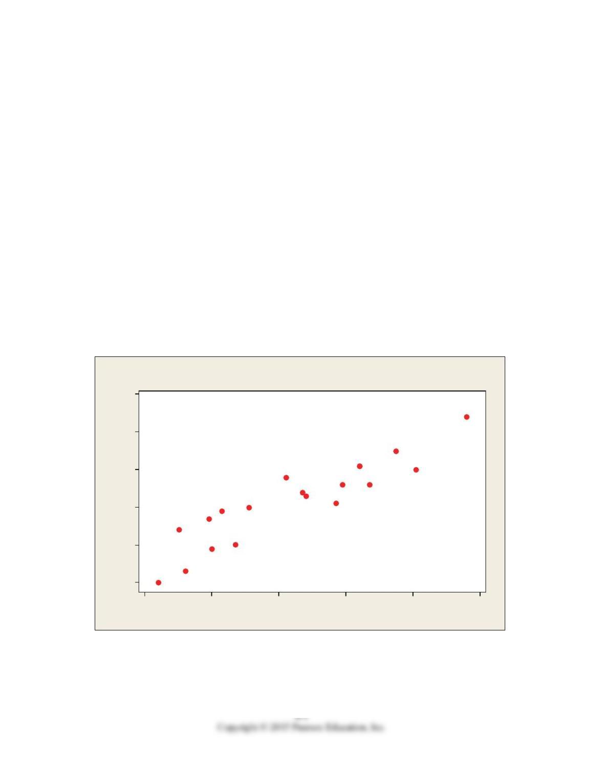
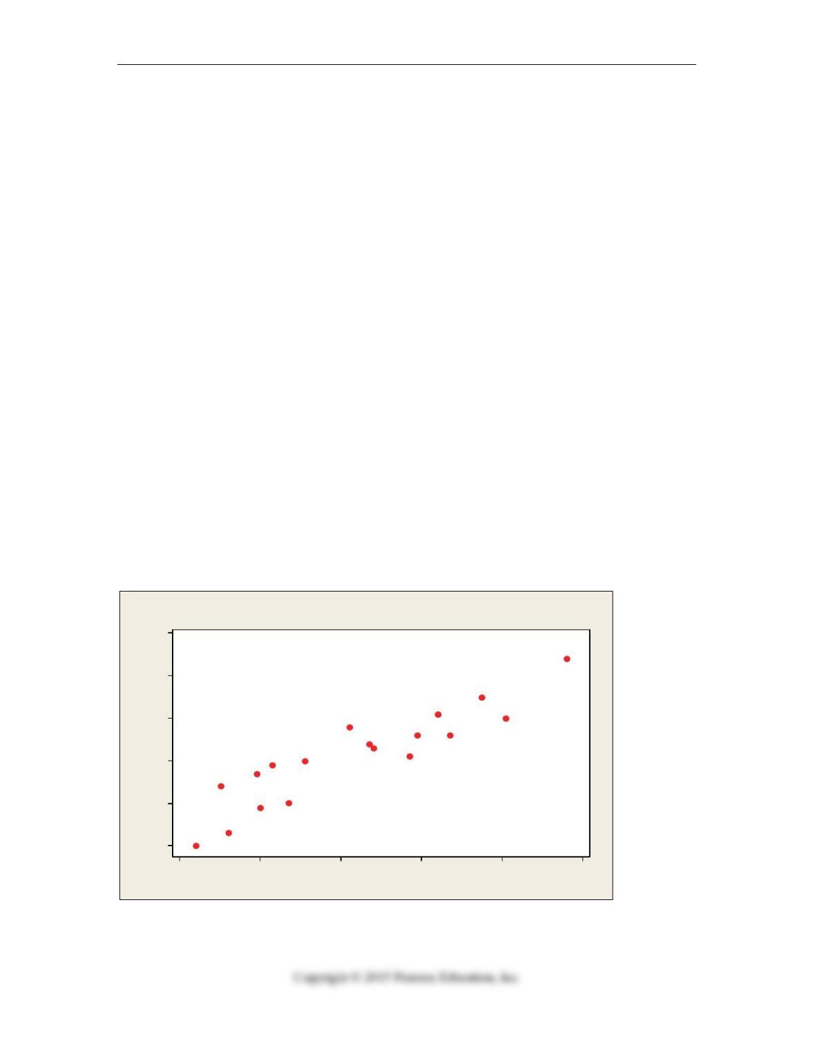
3. The following scatterplot shows monthly sales figures (in units) and number of
months of experience on the job for a sample of 19 salespeople.
100806040200
80
70
60
50
40
30
Exper ience
Sales
Scatterplot of Sales vs Experience
a. Describe the association between monthly sales and level of experience.
b. Do these data satisfy the conditions for computing a correlation coefficient? Explain.
c. Estimate the correlation.
4-2 Chapter 4 Correlation and Linear Regression
4.3.2 Summarize the strength of a linear relationship with a correlation, r.
4. Shown below is a correlation table showing correlation coefficients between stock
price, earnings per share (EPS), and price/earnings (P/E) ratio for a sample of 19 publicly
traded companies.
Correlations: Stock Price, EPS, PE
Stock Price EPS
EPS 0.875
PE 0.323 -0.111
a. What is the correlation between stock price and EPS? Interpret.
b. What is the correlation between stock price and PE? Interpret.
c. What is the correlation between EPS and PE? Interpret.
Use the following to answer questions 5 – 8.
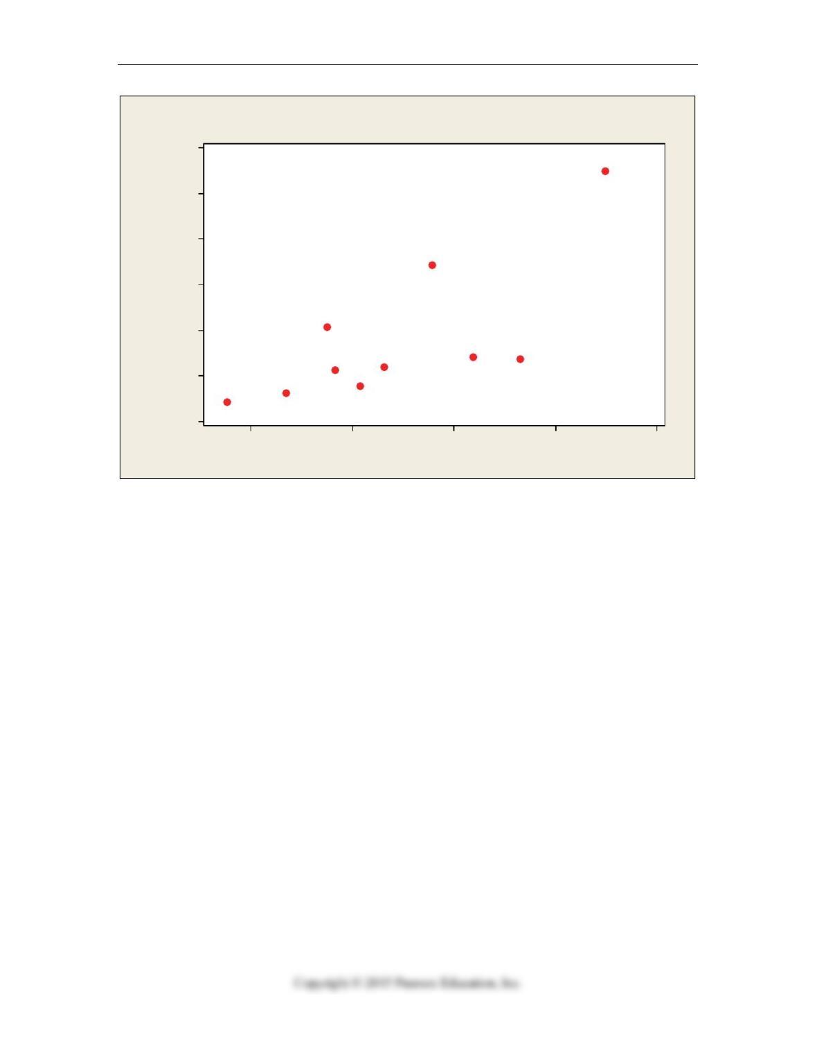
To determine whether the cash bonus paid by a company is related to annual pay, data
were gathered for 10 loan officers at AMC Bank who received cash bonuses in 2012.
The data, scatterplot, and summary statistics are shown below.
ANNUAL PAY CASH BONUS
$ 70609 $ 11225
$ 58487 $ 6238
$ 104561 $ 14194
$ 43922 $ 4188
$ 82613 $ 11863
$ 116250 $ 13671
$ 76751 $ 7758
$ 68513 $ 20760
$ 137000 $ 55000
$ 94469 $ 34368
Mean $ 85318 $ 17927
Standard Deviation $ 28077 $ 15618
Correlation 0.735
Quiz A 4-3
1500001250001000007500050000
60000
50000
40000
30000
20000
10000
0
Pay
Cash Bonus
Scatterplot of Cash Bonus vs Pay
4.3.3 Model a linear relationship with a least squares regression model.
5. Comment on whether each of the following conditions for correlation / linear
regression is met.
a. Quantitative variable condition.
b. Linearity condition.
c. Outlier condition.
4.3.3 Model a linear relationship with a least squares regression model.
6. Estimate the linear regression model that relates the response variable (cash bonus) to
the predictor variable (annual pay).
a. Find the slope of the regression line.
b. Find the intercept of the regression line.
c. Write the equation of the linear model.
4.3.3 Model a linear relationship with a least squares regression model.
7. Find the value of R2. Interpret its meaning in this context.
4.5.5 Examine the residuals from a linear model to assess the quality of the model.
8. Using the estimated regression equation,
a. Estimate the cash bonus for an executive at Johnson Financial earning $82, 613 a year.
b. What is the residual for this estimate? What does it mean?

4-4 Chapter 4 Correlation and Linear Regression
4.7.4 Recognize regression to the mean when it occurs in data.
9. A business executive taught his managers that praise is more effective than
punishment. He was challenged by one of the managers who said that in his experience
praising an employee for executing a task is typically followed by a lesser performance,
whereas yelling at an employee for bad execution is typically followed by improved
performance.
a. Explain this case in terms of a failure to appreciate regression toward the mean.
b. How might luck factor into the improvement or deterioration of performance?
Quiz A 4-5
Chapter 4: Correlation and Linear Regression – Quiz A – Key
4-6 Chapter 4 Correlation and Linear Regression
Quiz A 4-7
4-8 Chapter 4 Correlation and Linear Regression
Quiz A 4-9

4-10 Chapter 4 Correlation and Linear Regression
Chapter 4: Correlation and Linear Regression – Quiz B
Name_________________________
4.3.2 Summarize the strength of a linear relationship with a correlation, r.
1. In commenting on the increase in home foreclosures, a news reporter stated “there
appears to be a strong correlation between home foreclosures and job loss of the head of
household.” Comment on this statement.
4.2.1 Make a scatterplot to display the relationship between two quantitative variables.
2. For each of the following scenarios indicate which is the predictor variable and which
is the response variable.
a. A supermarket chain gathers data on the amount they spend on promotional material
(specials, coupons, etc.) and sales revenue generated each quarter.
b. Government-sponsored research investigated the relationship between number of hours
individuals spend on the Internet and age.
c. A real estate association conducted a study on home prices and economic strength for
different regions of the United States.
4.3.2 Summarize the strength of a linear relationship with a correlation, r.
3. Shown below is a correlation table showing correlation coefficients between
population (millions), migration rate of mobile subscriptions to smart phones (in %) and
smart phone penetration per capita (in %) for a sample of 15 countries.
Correlations: Population, Migration rate of mobile subscriptions, Smartphone penetration
Population Migration rate
Migration rate -0.266
Smartphone penetration -0.419 0.885
a. What is the correlation between migration rate of mobile subscriptions and population?
Interpret.
b. What is the correlation between smart phone penetration and population? Interpret.
c. What is the correlation between migration rate of mobile subscriptions and smart
phone penetration? Interpret.
Quiz B 4-11
4.3.2 Summarize the strength of a linear relationship with a correlation, r.
4. A consumer research group investigating the relationship between the price of meat
(per pound) and the fat content (grams) gathered data that produced the following
scatterplot.
12108642
20
15
10
5
0
Price/lb
Fa t Gr a ms
Scatterplot of Fat Grams vs Price/lb
a. Describe the association between the price of meat and fat content.
b. Estimate the correlation.
c. If the point in the lower left hand corner ($2.00 per pound, 6 grams of fat) is removed,
would the correlation become stronger or weaker or remain the same? Explain.
4-12 Chapter 4 Correlation and Linear Regression
Use the following to answer questions 5 – 8.
A small independent organic food store offers a variety of specialty coffees. To
determine whether price has an impact on sales, the managers kept track of how many
pounds of each variety of coffee were sold last month. The data, scatterplot, and
summary statistics are shown below.
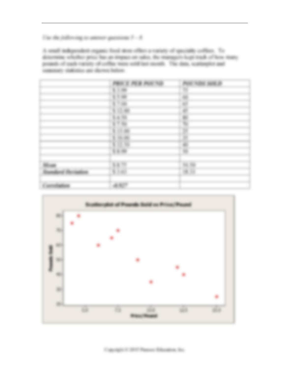
PRICE PER POUND POUNDS SOLD
$ 3.99 75
$ 5.99 60
$ 7.00 65
$ 12.00 45
$ 4.50 80
$ 7.50 70
$ 15.00 25
$ 10.00 35
$ 12.50 40
$ 8.99 50
Mean $ 8.75 54.50
Standard Deviation $ 3.63 18.33
Correlation -0.927
15.012.510.07.55.0
80
70
60
50
40
30
20
Price/Pound
Pounds Sold
Scatterplot of Pounds Sold vs Price/Pound

Quiz B 4-13
4.3.3 Model a linear relationship with a least squares regression model.
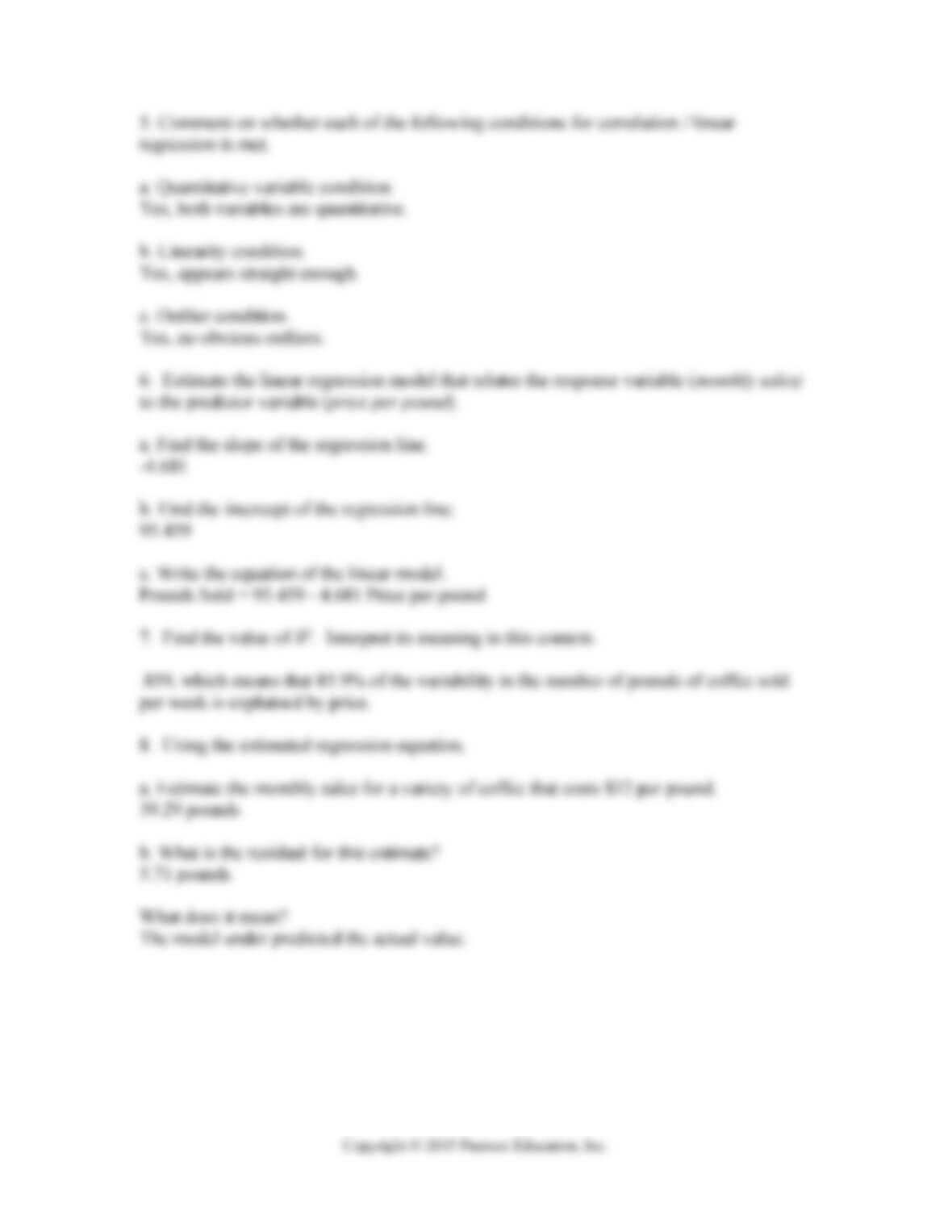
5. Comment on whether each of the following conditions for correlation / linear
regression is met.
a. Quantitative variable condition.
b. Linearity condition.
c. Outlier condition.
4.3.3 Model a linear relationship with a least squares regression model.
6. Estimate the linear regression model that relates the response variable (monthly sales)
to the predictor variable (price per pound).
a. Find the slope of the regression line.
b. Find the intercept of the regression line.
c. Write the equation of the linear model.
4.3.3 Model a linear relationship with a least squares regression model.
7. Find the value of R2. Interpret its meaning in this context.
4.5.5 Examine the residuals from a linear model to assess the quality of the model.
8. Using the estimated regression equation,
a. Estimate the monthly sales for a variety of coffee that costs $12 per pound.
b. What is the residual for this estimate? What does it mean?
4.7.4 Recognize regression to the mean when it occurs in data.
9. Some people believe that there is a Sports Illustrated cover jinx; that is, individuals or
teams who appear on the cover of Sports Illustrated will subsequently experience bad
luck.
a. Explain this case in terms of a failure to appreciate regression toward the mean.
b. Give an explanation for the deterioration in performance after the featured cover?
4-14 Chapter 4 Correlation and Linear Regression
Chapter 4: Correlation and Linear Regression – Quiz B – Key
Quiz B 4-15
4-16 Chapter 4 Correlation and Linear Regression
Quiz B 4-17
4-18 Chapter 4 Correlation and Linear Regression
Quiz C 4-19
Chapter 4: Correlation and Linear Regression – Quiz C – Multiple Choice
Name_________________________
4.2.1 Make a scatterplot to display the relationship between two quantitative variables.
1. A study examined consumption levels of oil and carbon dioxide emissions for
sample of counties. The response variable in this study is
A. oil.
B. oil consumption.
C. carbon dioxide emissions.
D. countries.
E. none of the above.
4.2.1 Make a scatterplot to display the relationship between two quantitative variables.
2. A supermarket chain gathers data on the amount they spend on promotional material
(e.g., coupons, etc.) and sales revenue generated each quarter. The predictor variable is
A. sales revenue.
B. amount spent on promotional material.
C. number of coupons offered.
D. supermarket chains.
E. none of the above.
4.3.2 Summarize the strength of a linear relationship with a correlation, r.
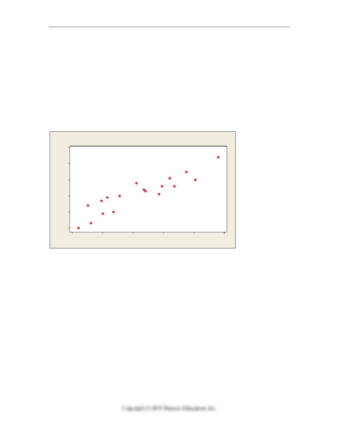
3. The scatterplot shows monthly sales figures (in units) and number of months of
experience for a sample of salespeople.
100806040200
80
70
60
50
40
30
Experience
Sales
Scatterplot of Sales vs Experience
4-20 Chapter 4 Correlation and Linear Regression
The association between monthly sales and level of experience can be described as
A. positive and weak.
B. negative and weak.
C. negative and strong.
D. positive and strong.
E. nonlinear.
4.3.2 Summarize the strength of a linear relationship with a correlation, r.
4. The scatterplot shows monthly sales figures (in units) and number of months of
experience for a sample of salespeople.
100806040200
80
70
60
50
40
30
Expe r ience
Sales
Scatterplot of Sales vs Experience
The correlation between monthly sales and level of experience is most likely
A. -.235.
B. 0.
C. .180.
D. -.914.
E. .914.
Quiz C 4-21
4.3.2 Summarize the strength of a linear relationship with a correlation, r.
5. Shown below is a correlation table showing correlation coefficients between stock
price, earnings per share (EPS) and price/earnings (P/E) ratio for a sample of 19
publicly traded companies. Which of the following statements is false?
Correlations: Stock Price, EPS, PE
Stock Price EPS
EPS 0.875
PE 0.323 -0.111
A. EPS is the best predictor of stock price.
B. The strongest correlation is between EPS and stock price.
C. There is a weak negative association between PE and EPS.
D. PE is the best predictor of stock price.
E. The weakest correlation is between PE and EPS.
4.2.1 Make a scatterplot to display the relationship between two quantitative variables.
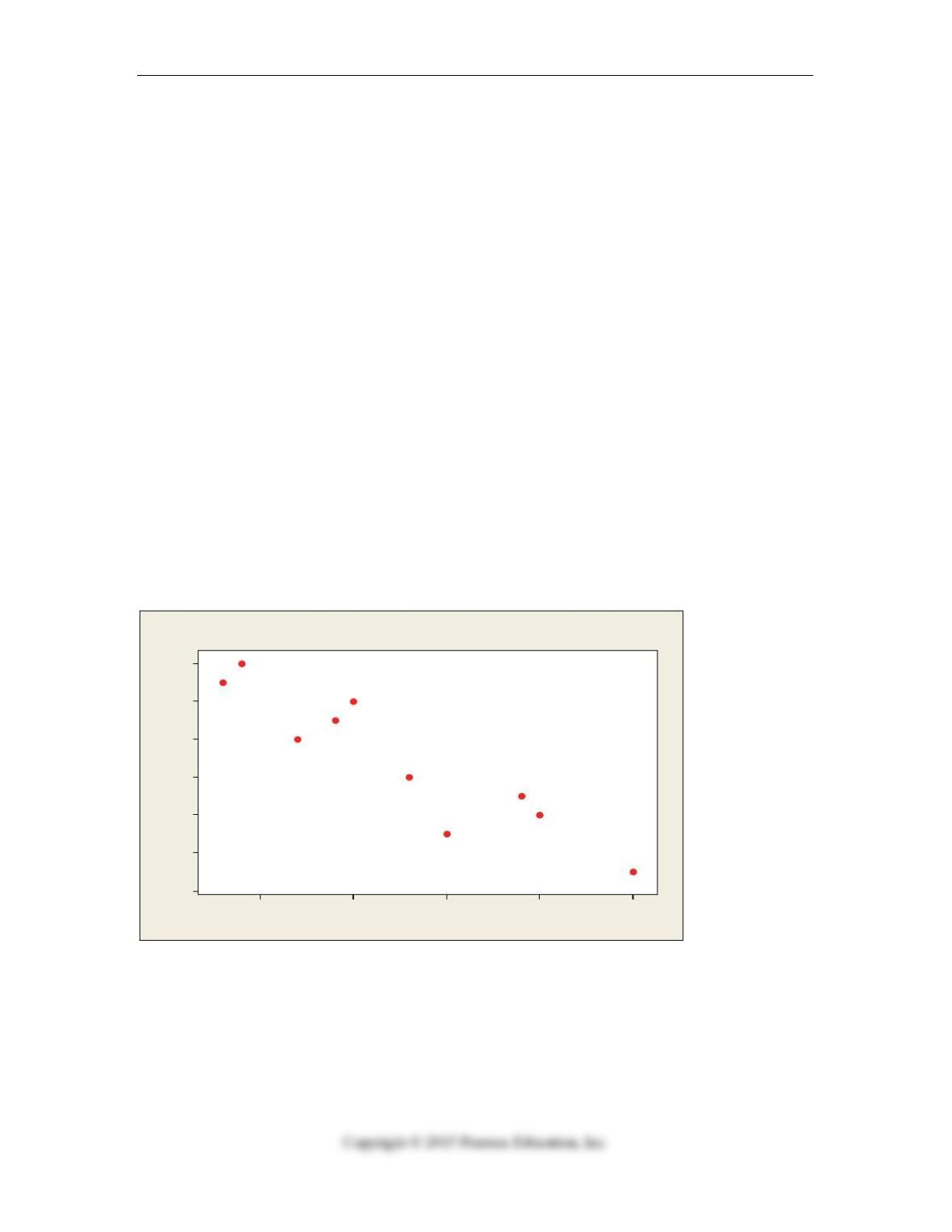
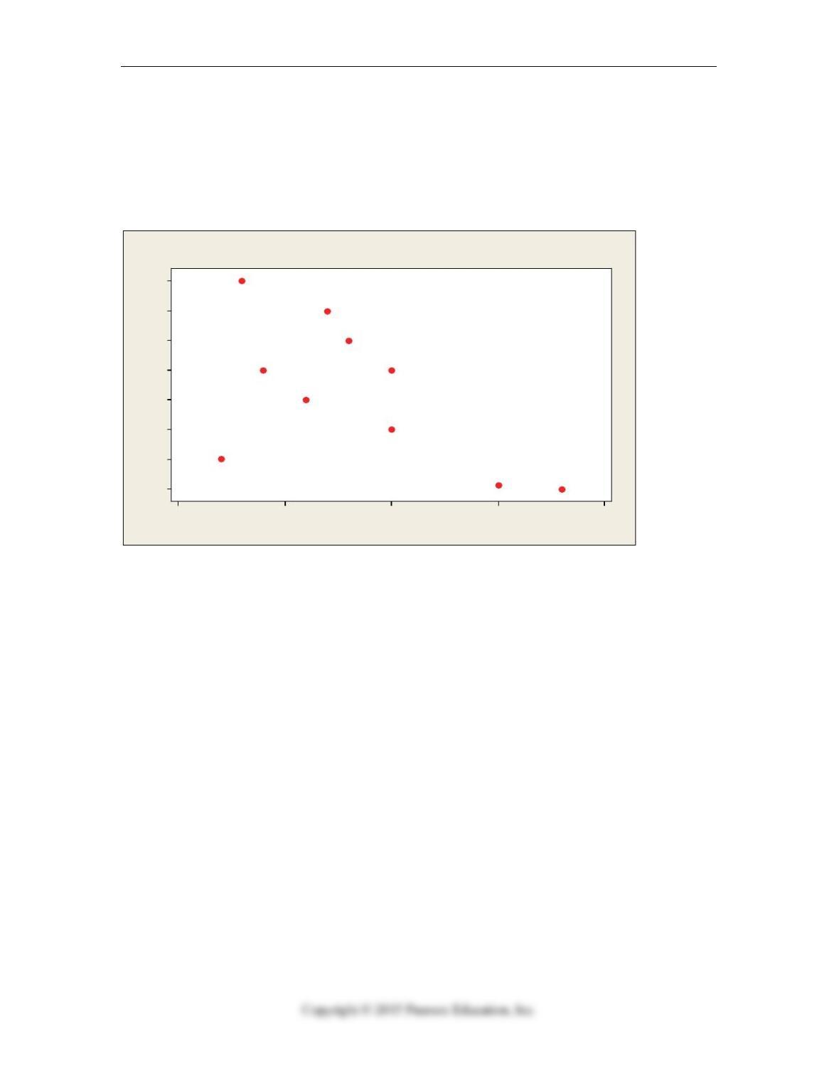
6. A small independent organic food store offers a variety of specialty coffees. To
determine whether price has an impact on sales, the managers kept track of how many
pounds of each variety of coffee were sold last month. Based on the scatterplot shown
below, which of the following statements is true?
15.012.510.07.55.0
80
70
60
50
40
30
20
Price/Pound
Pounds Sold
Scatterplot of Pounds Sold vs Price/Pound
A. The quantitative variable condition is satisfied.
B. The linearity condition is satisfied.
C. There are no obvious outliers.
D. All of the above.
E. None of the above.
4-22 Chapter 4 Correlation and Linear Regression
4.3.2 Summarize the strength of a linear relationship with a correlation, r.
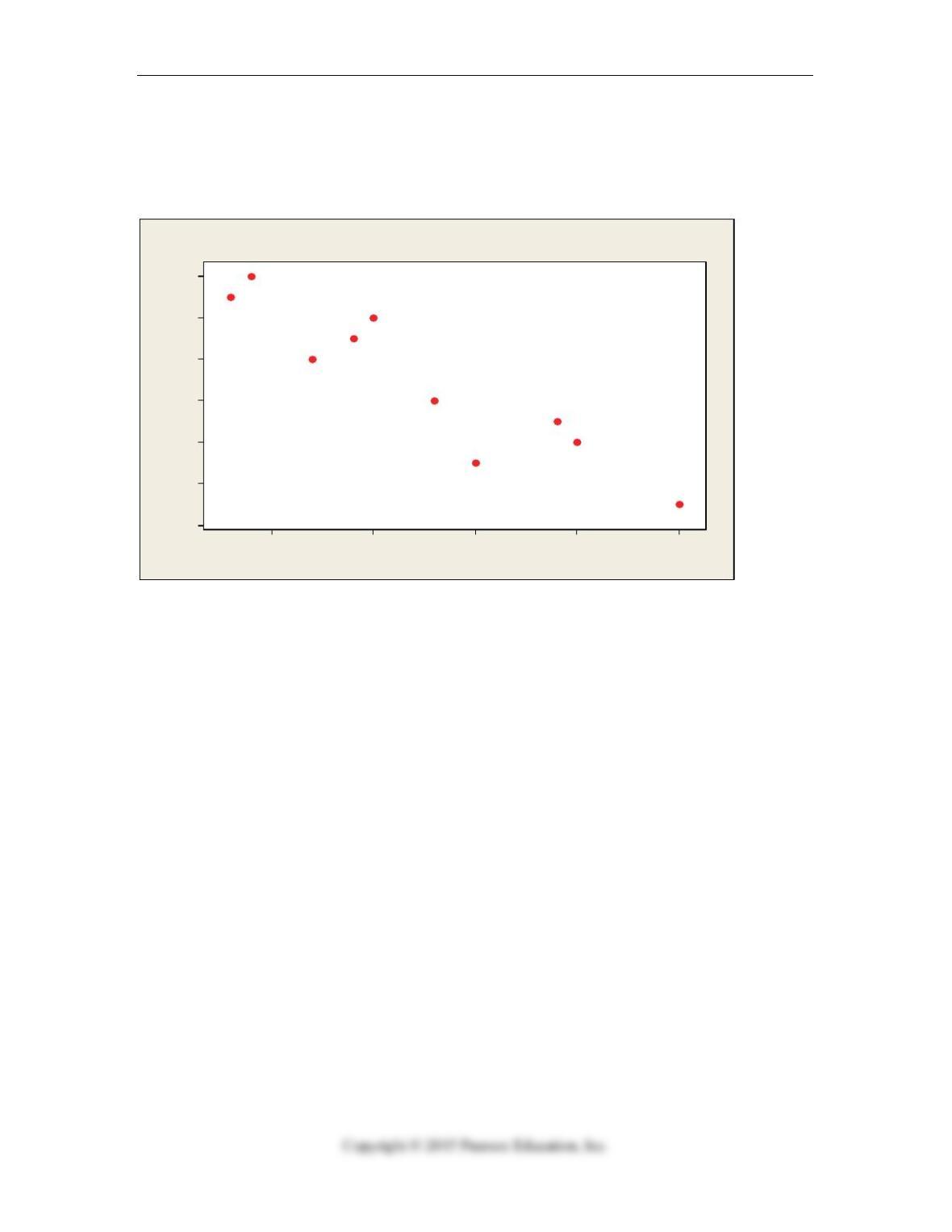
7. A small independent organic food store offers a variety of specialty coffees. To
determine whether price has an impact on sales, the managers kept track of how many
pounds of each variety of coffee were sold last month.
15.012.510.07.55.0
80
70
60
50
40
30
20
Price/Pound
Pounds Sold
Scatterplot of Pounds Sold vs Price/Pound
Based on the scatterplot, the linear relationship between number of pounds of coffee sold
per week and price is
A. strong and positive.
B. strong and negative.
C. weak and negative.
D. weak and positive.
E. nonexistent.
Quiz C 4-23
4.3.3 Model a linear relationship with a least squares regression model.
8. A small independent organic food store offers a variety of specialty coffees. To
determine whether price has an impact on sales, the managers kept track of how many
pounds of each variety of coffee were sold last month.
PRICE PER POUND POUNDS SOLD
$ 3.99 75
$ 5.99 60
$ 7.00 65
$ 12.00 45
$ 4.50 80
$ 7.50 70
$ 15.00 25
$ 10.00 35
$ 12.50 40
$ 8.99 50
Mean $ 8.75 54.50
Standard Deviation $ 3.63 18.33
Correlation -0.927
Based on the data and summary statistics shown below, the slope of the estimated
regression line that relates the response variable (monthly sales) to the predictor variable
(price per pound) is
A. 95. 459.
B. .858.
C. -4.681.
D. -.858.
E. -8.999.
4-24 Chapter 4 Correlation and Linear Regression
4.3.3 Model a linear relationship with a least squares regression model.
9. A small independent organic food store offers a variety of specialty coffees. To
determine whether price has an impact on sales, the managers kept track of how many
pounds of each variety of coffee were sold last month.
PRICE PER POUND POUNDS SOLD
$ 3.99 75
$ 5.99 60
$ 7.00 65
$ 12.00 45
$ 4.50 80
$ 7.50 70
$ 15.00 25
$ 10.00 35
$ 12.50 40
$ 8.99 50
Mean $ 8.75 54.50
Standard Deviation $ 3.63 18.33
Correlation -0.927
Based on the data and summary statistics, the intercept of the estimated regression line
that relates the response variable (monthly sales) to the predictor variable (price per
pound) is
A. 95.459.
B. .858.
C. -4.684.
D. -.858.
E. -8.999.
4.3.3 Model a linear relationship with a least squares regression model.
10. A small independent organic food store offers a variety of specialty coffees. To
determine whether price has an impact on sales, the managers kept track of how many
pounds of each variety of coffee were sold last month.
Based on the summary statistics shown below, what percent of the variability in the
number of pounds of coffee sold per week can be explained by price?
A. 95.47%
B. 100%
C. 85.9%
D. 55.6%
E. 4.68%
Mean $ 8.75 54.50
Standard Deviation $ 3.63 18.33
Correlation -0.927

Quiz C 4-25
4.6.11 Analyze and transform data in a nonlinear relationship.
11. A scatterplot shows a curved relationship between 2 variables. What methods can be
used to analyze the relationship between these variables?
A. Fit an exponential or quadratic function
B. Summarize the strength of the association by using ranks
C. Transform one or both of the variables by using square root, logarithm, or reciprocal
functions
D. A and C
E. All of the above
4-26 Chapter 4 Correlation and Linear Regression
Chapter 4: Correlation and Linear Regression – Quiz C – Key
Quiz D 4-27
Chapter 4: Correlation and Linear Regression – Quiz D – Multiple Choice
Name_________________________
4.1.1 Make a scatterplot to display the relationship between two quantitative variables.
1. A consumer research group examining the relationship between the price of meat (per
pound) and fat content (in grams) gathered data that produced the following scatterplot.
20151050
9
8
7
6
5
4
3
2
Fa t Gr a ms
Pr ice/lb
Scatterplot of Price/lb vs Fat Grams
If the point in the lower left hand corner (2 grams of fat; $3.00 per pound) is removed, the
correlation would most likely
A. remain the same.
B. become positive.
C. become weaker negative.
D. become stronger negative.
E. become zero.
4.3.6 Conditions for correlation; define and interpret linear regression; make predictions.
2. Data were collected on monthly sales revenues (in $1,000s) and monthly advertising
expenditures ($100s) for a sample of drug stores. The regression line relating revenues
(Y) to advertising expenditure (X) is estimated to be xy 00.93.48
ˆ+−= . The correct
interpretation of the slope is that for each additional
A. $1 spent on advertising, predicted sales revenue increases by $9,000.
B. $100 spent on advertising, predicted sales revenue increases by $9,000.
C. $100 spent on advertising, predicted sales revenue decreases by $9,000.
D. $1,000 in sales revenue, advertising expenditures decrease by $48.30.
E. $100 in sales revenue, advertising expenditures decrease by $48.30.

4-28 Chapter 4 Correlation and Linear Regression
4.3.3 Model a linear relationship with a least squares regression model.
3. Data were collected on monthly sales revenues (in $1,000s) and monthly advertising
expenditures ($100s) for a sample of drug stores. The regression line relating revenues
(Y) to advertising expenditure (X) is estimated to be xy 00.93.48
ˆ+−= . The predicted
sales revenue for a month in which $1,000 was spent on advertising is
A. $50,000.
B. $851.70.
C. $8,951.70.
D. $41,700.
E. $90,000.
4.3.3 Examine the residuals from a linear model to assess the quality of the model.
4. A company studying the productivity of its employees on a new information system
was interested in determining if the age (X) of data entry operators influenced the number
of completed entries made per hour (Y). The regression equation is xy 145.0374.14
ˆ−= .
Suppose the actual completed entries per hour for an operator who is 35 years old was 8.
The residual is
A. -1.3
B. 2.6
C. -3.5
D. 1.3
E. -2.2
4.3.6 Summarize the strength of a linear relationship with a correlation, r.
5. A company studying the productivity of their employees on a new information system
was interested in determining if the age (X) of data entry operators influenced the number
of completed entries made per hour (Y). The regression equation is xy 145.0374.14
ˆ−= .
If sx=14.04 and sy=2.61, then the correlation coefficient between age and productivity is
A. .779
B. -.236
C. .575
D. -.929
E. -.779
4.3.6 Summarize the strength of a linear relationship with a correlation, r.
6. Suppose the correlation, r, between two variables x and y is -0.44. What would you
predict about a y value if the x value is 2 standard deviations above its mean?
A. It will be .88 standard deviations below its mean.
B. It will be .88 standard deviations above its mean.
C. It will be 2 standard deviations below its mean.
D. It will be .44 standard deviations below its mean.
E. It will be .44 standard deviations above its mean.
Quiz D 4-29
4.3.9 Model a linear relationship with a least squares regression model.
7. Suppose the correlation, r, between two variables x and y is -0.44. What percentage of
the variability in y cannot be explained by x?
A. 19%
B. 44%
C. 81%
D. 88%
E. 12%
4.8.5 Examine the residuals from a linear model to assess the quality of the model.
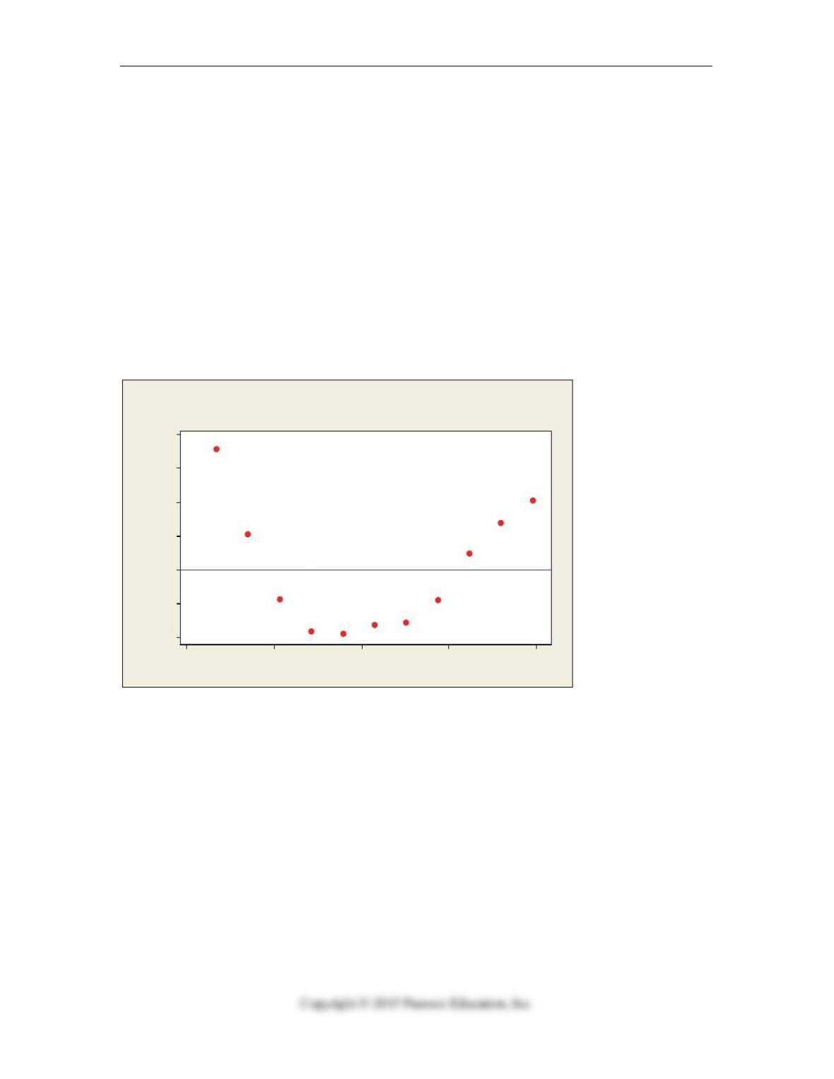
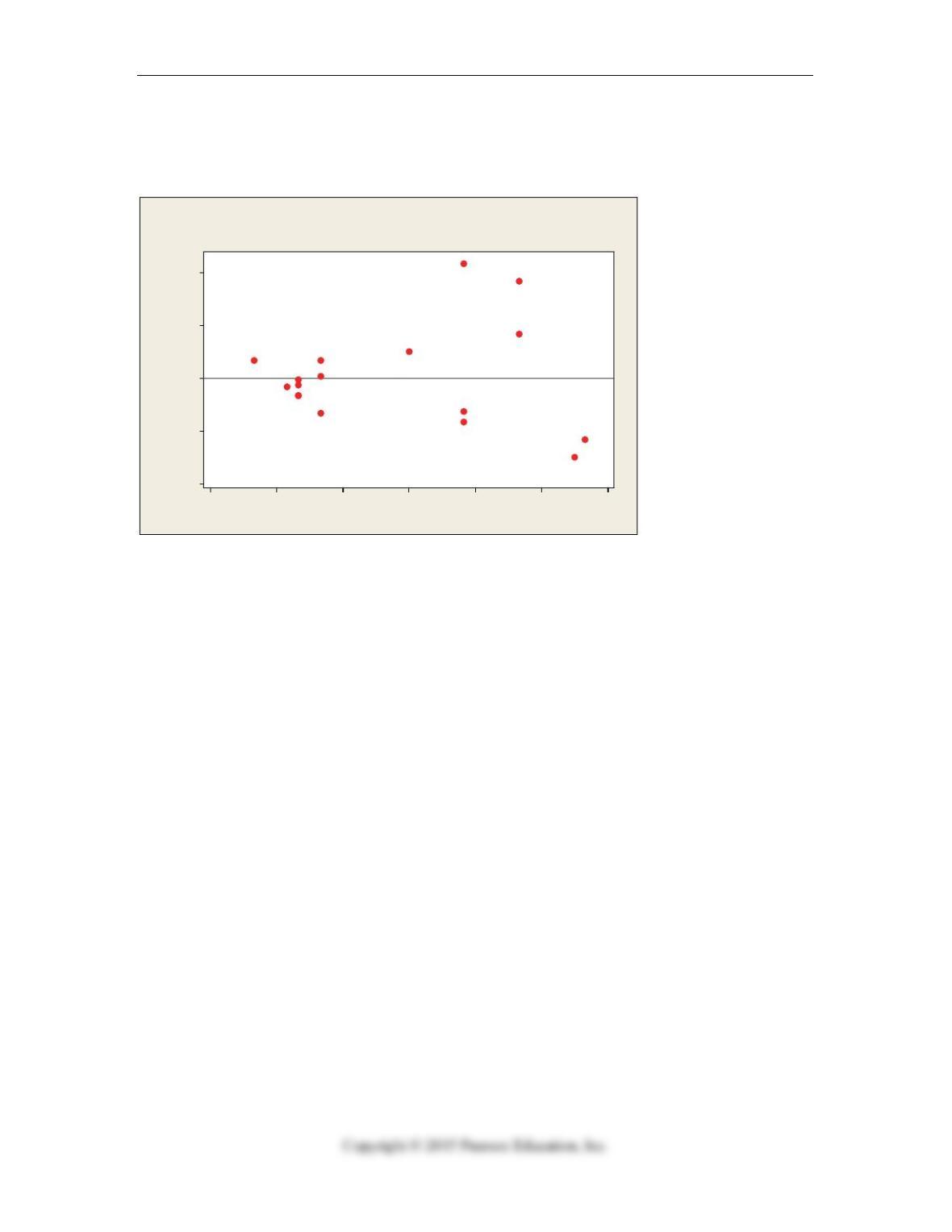
8. Linear regression was used to describe the trend in world population over time.
Below is a plot of the residuals versus predicted values. What does the plot of residuals
suggest?
60005000400030002000
200
150
100
50
0
-50
–100
Fit t e d V alu e
Residual
Versus Fits
(response is Population (millions))
A. An outlier is present in the data set.
B. The linearity condition is not satisfied.
C. A high leverage point is present in the data set.
D. The data are not normal.
E. The equal spread condition is not satisfied.
4-30 Chapter 4 Correlation and Linear Regression
4.8.5 Examine the residuals from a linear model to assess the quality of the model.
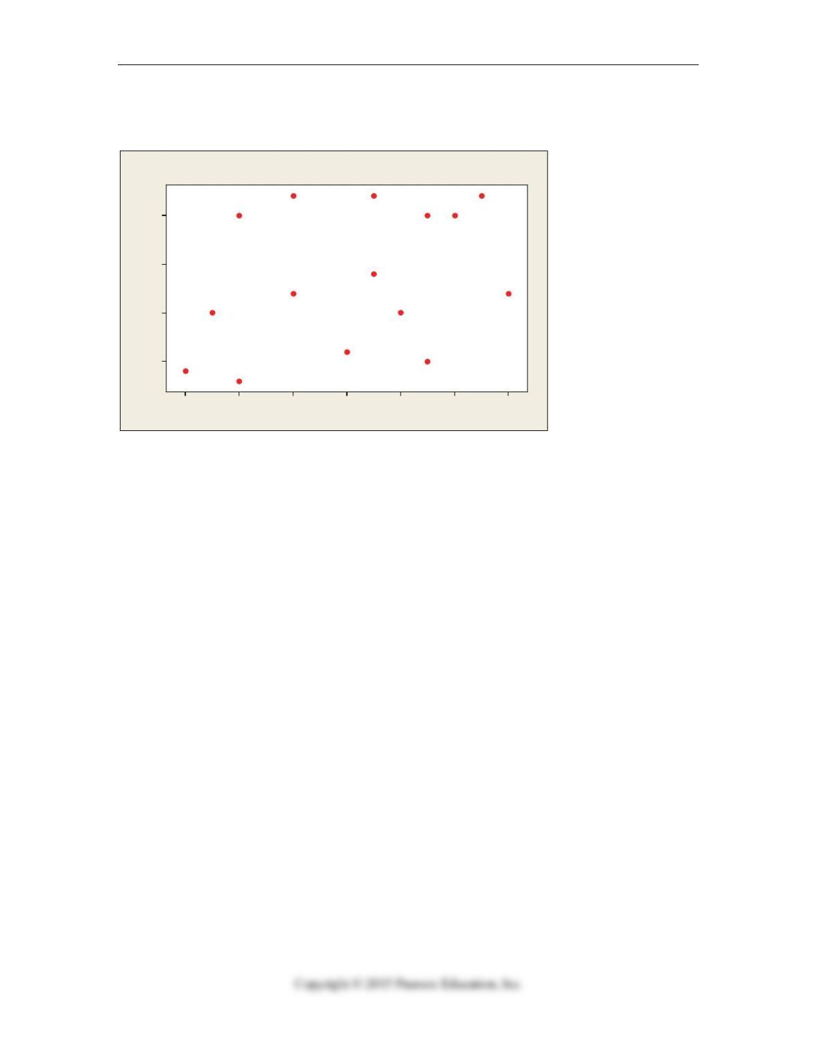
9. Based on the following residual plot, which condition / assumption for linear
regression is not satisfied?
700600500400300200100
200
100
0
-100
-200
Fit t e d V a lue
Residual
Versus Fits
(response is y)
A. Linearity.
B. Quantitative Variables.
C. Equal Spread.
D. Outlier.
E. None of the above; all conditions are satisfied.
Quiz D 4-31
4.3.2 Summarize the strength of a linear relationship with a correlation, r.
10. For the following scatterplot,
2018161412108
20
15
10
5
x
y
Scatterplot of y vs x
The likely correlation coefficient is
A. +0.35
B. +0.90
C. +0.77
D. -0.89
E. -1.00
4.11.6 Analyze and transform data in a nonlinear relationship.
11. The disadvantage of re-expressing variables is that
A. We have to explain the association in terms of the transformed variables.
B. We cannot use the standard regression models
C. It is not commonly used
D. It can be difficult
E. A and D
4-32 Chapter 4 Correlation and Linear Regression
Chapter 4: Correlation and Linear Regression – Quiz D – Key