Numerical Descriptive Measures 3-1
CHAPTER 3: NUMERICAL DESCRIPTIVE MEASURES
1. Which of the following statistics is not a measure of central tendency?
a) Arithmetic mean.
b) Median.
c) Mode.
d) Q3.
2. Which measure of central tendency can be used for both numerical and categorical variables?
a) Arithmetic mean.
b) Median.
c) Mode.
d) Geometric mean.
3. Which of the arithmetic mean, median, mode, and geometric mean are resistant measures of
central tendency?
a) The arithmetic mean and median only.
b) The median and mode only.
c) The mode and geometric mean only.
d) The arithmetic mean and mode only.
4. In a right-skewed distribution
a) the median equals the arithmetic mean.
b) the median is less than the arithmetic mean.
c) the median is greater than the arithmetic mean.
d) none of the above.
3-2 Numerical Descriptive Measures
5. Which of the following statements about the median is not true?
a) It is more affected by extreme values than the arithmetic mean.
b) It is a measure of central tendency.
c) It is equal to Q2.
d) It is equal to the mode in bell-shaped “normal” distributions.
6. In a perfectly symmetrical bell-shaped “normal” distribution
a) the arithmetic mean equals the median.
b) the median equals the mode.
c) the arithmetic mean equals the mode.
d) All the above.
7. In a perfectly symmetrical distribution
a) the range equals the interquartile range.
b) the interquartile range equals the arithmetic mean.
c) the median equals the arithmetic mean.
d) the variance equals the standard deviation.
8. When extreme values are present in a set of data, which of the following descriptive summary
measures are most appropriate:
a) CV and range.
b) arithmetic mean and standard deviation.
c) interquartile range and median.
d) variance and interquartile range.
Numerical Descriptive Measures 3-3
9. In general, which of the following descriptive summary measures cannot be easily approximated
from a boxplot?
a) The variance.
b) The range.
c) The interquartile range.
d) The median.
10. The smaller the spread of scores around the arithmetic mean,
a) the smaller the interquartile range.
b) the smaller the standard deviation.
c) the smaller the coefficient of variation.
d) All the above.
11. Which descriptive summary measures are considered to be resistant statistics?
a) The arithmetic mean and standard deviation.
b) The interquartile range and range.
c) The mode and variance.
d) The median and interquartile range.
12. In right-skewed distributions, which of the following is the correct statement?
a) The distance from Q1 to Q2 is greater than the distance from Q2 to Q3.
b) The distance from Q1 to Q2 is less than the distance from Q2 to Q3.
c) The arithmetic mean is less than the median.
d) The mode is greater than the arithmetic mean.
3-4 Numerical Descriptive Measures
13. In perfectly symmetrical distributions, which of the following is NOT a correct statement?
a) The distance from Q1 to Q2 equals to the distance from Q2 to Q3.
b) The distance from the smallest observation to Q1 is the same as the distance from Q3 to
the largest observation.
c) The distance from the smallest observation to Q2 is the same as the distance from Q2 to
the largest observation.
d) The distance from Q1 to Q3 is half of the distance from the smallest to the largest
observation.
14. In left-skewed distributions, which of the following is the correct statement?
a) The distance from Q1 to Q2 is smaller than the distance from Q2 to Q3.
b) The distance from the smallest observation to Q1 is larger than the distance from Q3 to the
largest observation.
c) The distance from the smallest observation to Q2 is less than the distance from Q2 to the
largest observation.
d) The distance from Q1 to Q3 is twice the distance from the Q1 to Q2.
15. According to the empirical rule, if the data form a “bell-shaped” normal distribution, _______
percent of the observations will be contained within 2 standard deviations around the arithmetic
mean.
a) 68.26
b) 88.89
c) 93.75
d) 95.44
Numerical Descriptive Measures 3-5
16. According to the empirical rule, if the data form a “bell-shaped” normal distribution, _______
percent of the observations will be contained within 1 standard deviation around the arithmetic
mean.
a) 68.26
b) 75.00
c) 88.89
d) 93.75
17. According to the empirical rule, if the data form a “bell-shaped” normal distribution, _______
percent of the observations will be contained within 3 standard deviations around the arithmetic
mean.
a) 68.26
b) 75.00
c) 95.0
d) 99.7
18. Which of the following is NOT a measure of central tendency?
a) The arithmetic mean.
b) The geometric mean.
c) The mode.
d) The interquartile range.
19. Which of the following is NOT sensitive to extreme values?
a) The range.
b) The standard deviation.
c) The interquartile range.
d) The coefficient of variation.
3-6 Numerical Descriptive Measures
20. Which of the following is sensitive to extreme values?
a) The median.
b) The interquartile range.
c) The arithmetic mean.
d) The 1st quartile.
21. Which of the following is the easiest to compute?
a) The arithmetic mean.
b) The median.
c) The mode.
d) The geometric mean.
22. According to the Chebyshev rule, at least 75% of all observations in any data set are contained
within a distance of how many standard deviations around the mean?
a) 1
b) 2
c) 3
d) 4
23. According to the Chebyshev rule, at least 93.75% of all observations in any data set are contained
within a distance of how many standard deviations around the mean?
a) 1
b) 2
c) 3
d) 4
Numerical Descriptive Measures 3-7
24. According to the Chebyshev rule, at least what percentage of the observations in any data set are
contained within a distance of 3 standard deviations around the mean?
a) 67%
b) 75%
c) 88.89%
d) 99.7%
25. According to the Chebyshev rule, at least what percentage of the observations in any data set are
contained within a distance of 2 standard deviations around the mean?
a) 67%
b) 75%
c) 88.89%
d) 95%
3-8 Numerical Descriptive Measures
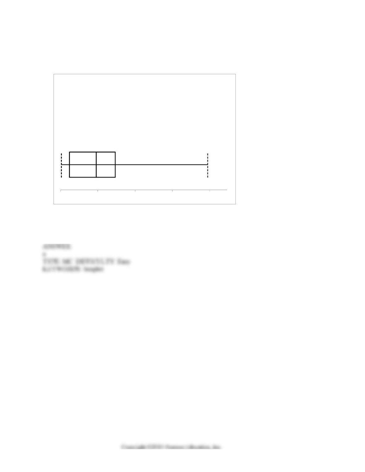
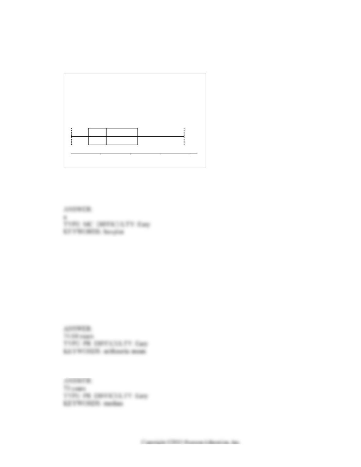
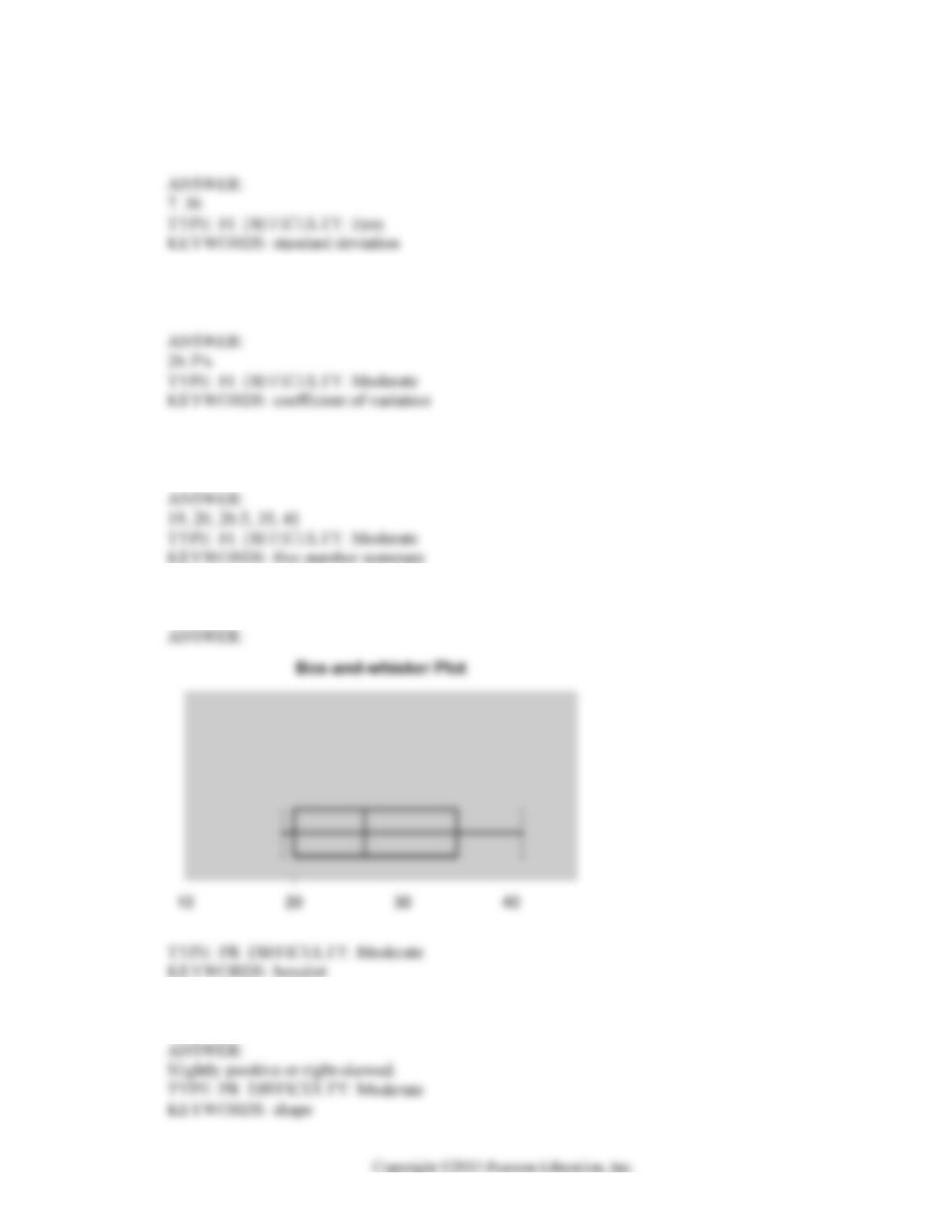
26. A manufacturer of flashlight batteries took a sample of 130 batteries from a day’s production and
used them continuously until they were drained. The number of hours until failure are recorded.
Given below is the boxplot of the number of hours it took to drain each of the 130 batteries. The
distribution of the number of hours is
a) right-skewed
b) left-skewed
c) symmetrical
d) none of the above
Hours
260 460 660 860 1060
Boxplot
Numerical Descriptive Measures 3-9
27. Data on the change in the cost of tuition, a shared dormitory room, and the most popular meal plan
from one academic year to the next academic year for a sample of 100 public universities are
collected. Below is the boxplot for the change in cost in dollars. The distribution of the change in
cost is
a) right-skewed
b) left-skewed
c) symmetrical
d) none of the above
SCENARIO 3-1
Health care issues are receiving much attention in both academic and political arenas. A sociologist
recently conducted a survey of citizens over 60 years of age whose net worth is too high to qualify for
Medicaid. The ages of 25 senior citizens were as follows:
60 61 62 63 64 65 66 68 68 69 70 73 73
74 75 76 76 81 81 82 86 87 89 90 92
28. Referring to Scenario 3-1, calculate the arithmetic mean age of the senior citizens to the nearest
hundredth of a year.
29. Referring to Scenario 3-1, determine the median age of the senior citizens.
Change in
Cost ($)
300 800 1300 1800 2300
Boxplot
3-10 Numerical Descriptive Measures
30. Referring to Scenario 3-1 determine the first quartile of the ages of the senior citizens.
31. Referring to Scenario 3-1 determine the third quartile of the ages of the senior citizens.
32. Referring to Scenario 3-1, determine the interquartile range of the ages of the senior citizens.
33. Referring to Scenario 3-1, determine which of the following is the correct statement.
a) One fourth of the senior citizens sampled are below 65.5 years of age.
b) The middle 50% of the senior citizens sampled are between 65.5 and 73.0 years of age.
c) The mean age of senior citizens sampled is 73.5 years of age.
d) All of the above are correct.
34. Referring to Scenario 3-1, identify which of the following is the correct statement.
a) One fourth of the senior citizens sampled are below 64 years of age.
b) The middle 50% of the senior citizens sampled are between 65.5 and 73.0 years of age.
c) 25% of the senior citizens sampled are older than 81.5 years of age.
d) All of the above are correct.
35. Referring to Scenario 3-1, calculate the skewness statistic for the age of the senior citizens
accurate to two decimal places.
Numerical Descriptive Measures 3-11
36. Referring to Scenario 3-1, what type of shape does the distribution of the sample appear to have?
37. Referring to Scenario 3-1, calculate the kurtosis statistic for the age of the senior citizens accurate
to two decimal places.
38. Referring to Scenario 3-1, does the distribution of the sample appear to be lepokurtic or
platykurtic?
39. Referring to Scenario 3-1, calculate the variance of the ages of the senior citizens correct to the
nearest hundredth of a year squared.
40. Referring to Scenario 3-1, calculate the standard deviation of the ages of the senior citizens
correct to the nearest hundredth of a year.
41. Referring to Scenario 3-1, calculate the coefficient of variation of the ages of the senior citizens.
3-12 Numerical Descriptive Measures
42. True or False: The median of the values 3.4, 4.7, 1.9, 7.6, and 6.5 is 1.9.
43. True or False: The median of the values 3.4, 4.7, 1.9, 7.6, and 6.5 is 4.05.
44. True or False: In a set of numerical data, the value for Q3 can never be smaller than the value for
Q1.
45. True or False: In a set of numerical data, the value for Q2 is always halfway between Q1 and Q3.
46. True or False: If the distribution of a data set were perfectly symmetrical, the distance from Q1 to
the median would always equal the distance from Q3 to the median in a boxplot.
47. True or False: In right-skewed distributions, the distance from Q3 to the largest value is greater
than the distance from the smallest observation to Q1.
Numerical Descriptive Measures 3-13
48. True or False: In left-skewed distributions, the distance from the smallest value to Q1 is greater
than the distance from Q3 to the largest value.
49. True or False: A boxplot is a graphical representation of a five-number summary.
50. True or False: The five-number summary consists of the smallest value, the first quartile, the
median, the third quartile, and the largest value.
51. True or False: In a boxplot, the box portion represents the data between the first and third quartile
values.
52. True or False: The line drawn within the box of the boxplot always represents the arithmetic
mean.
53. True or False: The line drawn within the box of the boxplot always represents the median.
3-14 Numerical Descriptive Measures
54. True or False: In a sample of size 40, the sample mean is 15. In this case, the sum of all
observations in the sample is ∑
X
i = 600.
55. True or False: A population with 200 elements has an arithmetic mean of 10. From this
information, it can be shown that the population standard deviation is 15.
56. True or False: In exploratory data analysis, a boxplot can be used to illustrate the median,
quartiles, and extreme values.
57. True or False: The median of a data set with 20 items would be the average of the 10th and the
11th items in the ordered array.
58. True or False: The coefficient of variation measures variability in a data set relative to the size of
the arithmetic mean.
59. True or False: The coefficient of variation is expressed as a percentage.
Numerical Descriptive Measures 3-15
60. True or False: The coefficient of variation is a measure of central tendency in the data.
61. True or False: The interquartile range is a measure of variation or dispersion in a set of data.
62. True or False: The interquartile range is a measure of central tendency in a set of data.
63. True or False: The geometric mean is a measure of variation or dispersion in a set of data.
64. True or False: The geometric mean is useful in measuring the rate of change of a variable over
time.
65. True or False: If a set of data is perfectly symmetrical, the arithmetic mean must be identical to
the median.
66. True or False: The coefficient of variation is a measure of relative variation.
3-16 Numerical Descriptive Measures
67. True or False: If the data set is approximately bell-shaped, the empirical rule will more accurately
reflect the greater concentration of data close to the mean as compared to the Chebyshev rule.
68. If the arithmetic mean of a numerical data set is greater than the median, the data are considered
to be _______ skewed.
SCENARIO 3-2
The data below represent the amount of grams of carbohydrates in a serving of breakfast cereal in a
sample of 11 different servings.
11 15 23 29 19 22 21 20 15 25 17
69. Referring to Scenario 3-2, the arithmetic mean carbohydrates in this sample is ________ grams.
70. Referring to Scenario 3-2, the median carbohydrate amount in the cereal is ________ grams.
71. Referring to Scenario 3-2, the skewness statistic for the carbohydrate amount in the cereal is
________.
72. Referring to Scenario 3-2, is the carbohydrate amount in the cereal right- or left-skewed?
Numerical Descriptive Measures 3-17
73. Referring to Scenario 3-2, the kurtosis statistic for the carbohydrate amount in the cereal is
________.
74. Referring to Scenario 3-2, is the carbohydrate amount in the cereal leptokurtic or platykurtic?
75. Referring to Scenario 3-2, the first quartile of the carbohydrate amounts is ________ grams.
76. Referring to Scenario 3-2, the third quartile of the carbohydrate amounts is ________ grams.
77. Referring to Scenario 3-2, the range in the carbohydrate amounts is ________ grams.
78. Referring to Scenario 3-2, the interquartile range in the carbohydrate amounts is ________ grams.
79. Referring to Scenario 3-2, the variance of the carbohydrate amounts is ________ (grams
squared).
3-18 Numerical Descriptive Measures
80. Referring to Scenario 3-2, the standard deviation of the carbohydrate amounts is ________
grams.
81. Referring to Scenario 3-2, the coefficient of variation of the carbohydrate amounts is ________
percent.
82. Referring to Scenario 3-2, the five-number summary of the carbohydrate amounts consists of
________, ________, ________, ________, ________.
83. Referring to Scenario 3-2, construct a boxplot for the carbohydrate amounts.
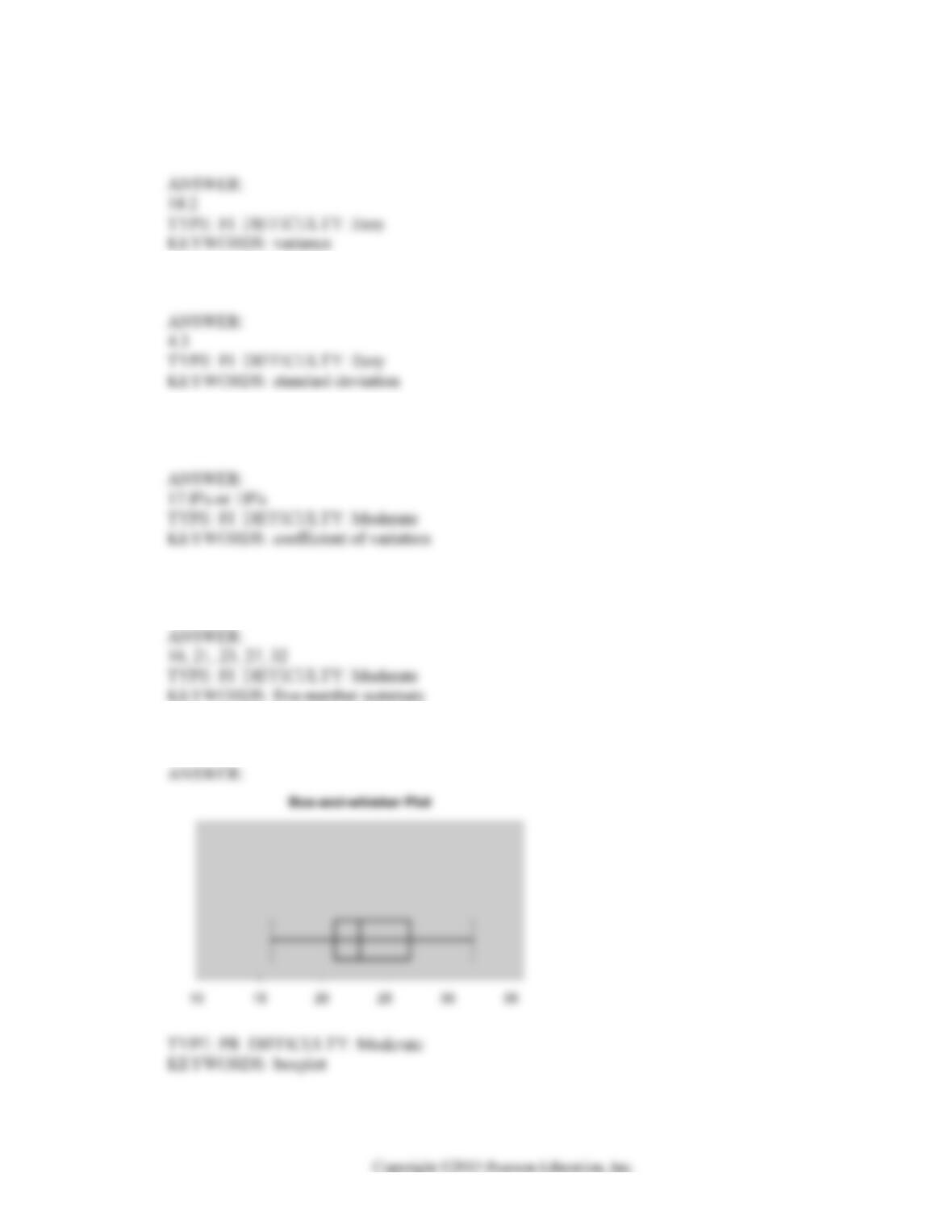
Numerical Descriptive Measures 3-19
SCENARIO 3-3
The ordered array below represents the number of vitamin supplements sold by a health food store in
a sample of 16 days.
19, 19, 20, 20, 22, 23, 25, 26, 27, 30, 33, 34, 35, 36, 38, 41
Note: For this sample, the sum of the values is 448, and the sum of the squared differences between
each value and the mean is 812.
84. Referring to Scenario 3-3, the arithmetic mean of the number of vitamin supplements sold in this
sample is ________.
85. Referring to Scenario 3-3, the first quartile of the number of vitamin supplements sold in this
sample is ________.
86. Referring to Scenario 3-3, the third quartile of the number of vitamin supplements sold in this
sample is ________.
87. Referring to Scenario 3-3, the median number of vitamin supplements sold in this sample is
________.
88. Referring to Scenario 3-3, the skewness statitic of the number of vitamin supplements sold in this
sample is ________.
3-20 Numerical Descriptive Measures
89. Referring to Scenario 3-3, is the number of vitamin supplements sold in this sample right- or left-
skewed?
90. Referring to Scenario 3-3, the kurtosis statitic of the number of vitamin supplements sold in this
sample is ________.
91. Referring to Scenario 3-3, is the number of vitamin supplements sold in this sample lepokurtic or
platykurtic?
92. Referring to Scenario 3-3, the range of the number of vitamin supplements sold in this sample is
________.
93. Referring to Scenario 3-3, the interquartile range of the number of vitamin supplements sold in
this sample is ________.
94. Referring to Scenario 3-3, the variance of the number of vitamin supplements sold in this sample
is ________.
Numerical Descriptive Measures 3-21
95. Referring to Scenario 3-3, the standard deviation of the number of vitamin supplements sold in
this sample is ________.
96. Referring to Scenario 3-3, the coefficient of variation of the number of vitamin supplements sold
in this sample is ________ percent.
97. Referring to Scenario 3-3, the five-number summary of the data in this sample consists of
________, ________, ________, ________, ________.
98. Referring to Scenario 3-3, construct a boxplot for the data in this sample.
99. Referring to Scenario 3-3, what type of shape does the distribution of the sample appear to have?
3-22 Numerical Descriptive Measures
SCENARIO 3-4
The ordered array below represents the number of cargo manifests approved by customs inspectors of
the Port of New York in a sample of 35 days:
16, 17, 18, 18, 19, 20, 20, 21, 21, 21, 22, 22, 22, 22, 23, 23, 23, 23, 24, 24, 24, 25, 25, 26, 26, 26, 27,
28, 28, 29, 29, 31, 31, 32, 32
Note: For this sample, the sum of the values is 838, , and the sum of the squared differences between
each value and the mean is 619.89.
100. Referring to Scenario 3-4, the arithmetic mean of the customs data is ________.
101. Referring to Scenario 3-4, the median of the customs data is ________.
102. Referring to Scenario 3-4, the first quartile of the customs data is ________.
103. Referring to Scenario 3-4, the third quartile of the customs data is ________.
104. Referring to Scenario 3-4, the range of the customs data is ________.
105. Referring to Scenario 3-4, the interquartile range of the customs data is ________.
Numerical Descriptive Measures 3-23
106. Referring to Scenario 3-4, the variance of the customs data is ________.
107. Referring to Scenario 3-4, the standard deviation of the customs data is ________.
108. Referring to Scenario 3-4, the coefficient of variation of the customs data is ________
percent.
109. Referring to Scenario 3-4, the five-number summary for the data in the customs sample
consists of ________, ________, ________, ________, ________.
110. Referring to Scenario 3-4, construct a boxplot of this sample.
3-24 Numerical Descriptive Measures
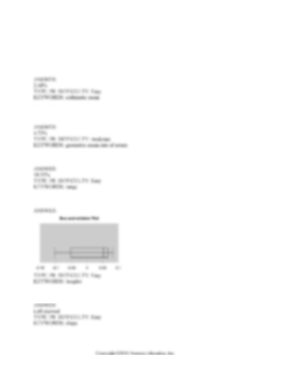
SCENARIO 3-5
The rate of return of a Fortune 500 company over the past 15 years are: 3.17%, 4.43%, 5.93%, 5.43%,
7.29%, 8.21%, 6.23%, 5.23%, 4.34%, 6.68%, 7.14%, -5.56%, -5.23%, -5.73%, -10.34%
111. Referring to Scenario 3-5, compute the arithmetic mean rate of return per year.
112. Referring to Scenario 3-5, compute the geometric mean rate of return per year for the first four
years.
113. Referring to Scenario 3-5, what is the range of the rate of return?
114. Referring to Scenario 3-5, construct a boxplot for the rate of return.
115. Referring to Scenario 3-5, what is the shape of the distribution for the rate of return?
Numerical Descriptive Measures 3-25
SCENARIO 3-6
The rate of return of an Internet Service Provider over a 10 year period are: 10.25%, 12.64%, 8.37%,
9.29%, 6.23%, 42.53%, 29.23%, 15.25%, 21.52%, -2.35%.
116. Referring to Scenario 3-6, compute the arithmetic mean rate of return per year.
117. Referring to Scenario 3-6, compute the geometric mean rate of return per year for the first three
years.
118. Referring to Scenario 3-6, construct a boxplot for the rate of return
119. Referring to Scenario 3-6, what is the shape of the distribution for the rate of return?
120. You were told that the 1st, 2nd and 3rd quartiles of female students’ weight at a major university
are 95 lbs, 125 lbs, and 138 lbs. What percentage of the students weigh more than 138 lbs?
3-26 Numerical Descriptive Measures
121. You were told that the 1st, 2nd and 3rd quartiles of female students’ weight at a major university
are 95 lbs, 125 lbs, and 138 lbs. What percentage of the students weigh less than 95 lbs?
122. You were told that the 1st, 2nd and 3rd quartiles of female students’ weight at a major university
are 95 lbs, 125 lbs, and 138 lbs. What percentage of the students weigh between 95 and 138 lbs?
123. You were told that the 1st, 2nd and 3rd quartiles of female students’ weight at a major university
are 95 lbs, 125 lbs, and 138 lbs. What percentage of the students weigh more than 125 lbs?
124. The Z scores can be used to identify outliers.
125. The larger the Z score, the farther is the distance from the value to the median.
126. As a general rule, a value is considered an extreme value if its Z score is greater than −3.
127. As a general rule, a value is considered an extreme value if its Z score is greater than 3.
Numerical Descriptive Measures 3-27
128. As a general rule, a value is considered an extreme value if its Z score is less than 3.
129. As a general rule, a value is considered an extreme value if its Z score is less than −3.
130. The Z score of a value can never be negative.
131. The Z score of a value measures how many standard deviations the value is from the mean.
132. The 12-month rate of returns over a three year period of a particular stock is 0.099, −0.289, and
0.089. The geometric mean rate of return per year for this stock is _______.
133. The rate of return for the S&P 500 over a four year period is −0.029, −0.061, −0.493, and
−0.286. The geometric mean rate of return per year is _______.
134. The rate of return for a stock over a three year period is 0.527, 0.145, and 0.684. The geometric
mean rate of return is _______.
3-28 Numerical Descriptive Measures
SCENARIO 3-7
In a recent academic year, many public universities in the United States raised tuition and fees due to
a decrease in state subsidies. The change in the cost of tuition, a shared dormitory room, and the most
popular meal plan from the previous academic year for a sample of 10 public universities were as
follows: $1,589, $593, $1,223, $869, $423, $1,720, $708, $1425, $922 and $308.
135. Referring to Scenario 3-7, what is the mean and median change in the cost?
136. Referring to Scenario 3-7, what is the five-number summary of the change in the cost?
137. Referring to Scenario 3-7, what is the standard deviation of the change in the cost?
138. Referring to Scenario 3-7, what is the interquartile range of the change in the cost?
139. Referring to Scenario 3-7, what is the coefficient of variation of the change in cost?
140. Referring to Scenario 3-7, what is the skewness statistic of the change in the cost?
Numerical Descriptive Measures 3-29
141. Referring to Scenario 3-7, is the change in the cost right- or left-skewed?
142. Referring to Scenario 3-7, what is the kurtosis statistic of the change in the cost?
143. Referring to Scenario 3-7, is the change in the cost lepokurtic or platykurtic?
144. Referring to Scenario 3-7, what are the (absolute values of) the Z scores of the change in cost?
145. Referring to Scenario 3-7, are the data skewed? If so, how?
3-30 Numerical Descriptive Measures
SCENARIO 3-8
The time period from 2010 to 2013 saw a great deal of volatility in the value of stocks. The data in
the following table represent the total rate of return of our companies from 2010 to 2013.
Year Company A Company B Company C Company D
2013 25.30 26.40 45.40 29.40
2012 -15.01 -22.10 -21.58 -20.90
2011 -5.44 -11.90 -1.03 -10.97
2010 -6.20 -9.10 -3.02 -10.89
146. Referring to Scenario 3-8, calculate the geometric mean rate of return per year for Company A.
147. Referring to Scenario 3-8, calculate the geometric mean rate of return per year for Company B.
148. Referring to Scenario 3-8, calculate the geometric mean rate of return per year for Company C.
149. Referring to Scenario 3-8, calculate the geometric mean rate of return per year for Company D.
Numerical Descriptive Measures 3-31
SCENARIO 3-9
The following table represents the assets in billions of dollars of the five largest bond funds sometime
in the past.
Bond Fund Assets (Billions $)
PIMCO Total Return Fund 246
Vanguard Total Bond Market Index Fund 110
Templeton Global Bond Fund 57
Vanguard Total Bond Market Index Fund II 56
Vanguard Inflation-Protected Securities 43
150. Referring to Scenario 3-9, what is the mean for this population of the five largest bond funds?
151. Referring to Scenario 3-9, what are the variance and standard deviation for this population?
SCENARIO 3-10
The population of eight analysts at a software firm were asked to estimate the reuse rate when
developing a new software system. The following data are given as a percentage of the total code
written for a software system that is part of the reuse database.
50, 62.5, 37.5, 75.0, 45.0, 47.5, 15.0, 25.0
152. Referring to Scenario 3-10, what is the mean percentage of the total code that is part of the
reuse database?
153. Referring to Scenario 3-10, what are the variance and standard deviation of the total code that is
part of the reuse database?
3-32 Numerical Descriptive Measures
SCENARIO 3-11
Given below are the closing prices for the Dow Jones Industrial Average (DJIA) and the Standard &
Poor’s (S&P) 500 Index over a 10-week sometime in the past.
Dow Jones 10,421 10,110 9,862 10,475 9,920 10,592 11,213 10,933 11,134 10,316
S&P 500 1,379 1,356 1,343 1,410 1,389 1,463 1,529 1,499 1,516 1,355
154. Referring to Scenario 3-11, what is the sample covariance between the DJIA and the S&P 500
index?
155. Referring to Scenario 3-11, what is the sample correlation coefficient between the DJIA and the
S&P 500 index?
156. Referring to Scenario 3-11, how will you classify the linear relationship between the DJIA and
the S&P 500 index?
a) Weak
b) Moderate
c) Strong
d) No relationship
157. Referring to Scenario 3-11, for the week when the DJIA is high, you will expect the S&P index
in that week to
a) be about the same value as the DJIA
b) be low
c) be high
d) have no relationship with the DJIA value
Numerical Descriptive Measures 3-33
158. Referring to Scenario 3-11, you will expect an increase in the DJIA to be associated with
a) an increase in the S&P 500 index
b) a decrease in the S&P 500 index
c) no predictable change in the DJIA
d) no predictable change in the S&P 500 index
SCENARIO 3-12
Given below are the rating and performance scores of 15 laptop computers.
Performance
Score
115 191 153 194 236 184 184 216
Overall
Rating
74 78 79 80 84 76 77 92
Performance
Score
185 183 189 202 192 141 187
Overall
Rating
83 78 77 78 78 73 77
159. Referring to Scenario 3-12, what is the sample covariance between the performance scores and
the rating?
160. Referring to Scenario 3-12, what is the sample correlation coefficient between the performance
scores and the rating?
3-34 Numerical Descriptive Measures
161. Referring to Scenario 3-12, how will you classify the linear relationship between the
performance scores and the rating?
a) Weak
b) Moderate
c) Strong
d) No relationship
162. Referring to Scenario 3-12, for a laptop computer that has a high rating, you will expect its
performance score to
a) be about the same as its rating
b) be low
c) be high
d) have no relationship with its rating
163. Referring to Scenario 3-12, you will expect a decrease in the performance score of one laptop
computer to be associated with
a) an increase in its rating
b) a decrease in its rating
c) no predictable change in its rating
d) no predictable change in the performance score of another laptop computer
Numerical Descriptive Measures 3-35
SCENARIO 3-13
Energy drink consumption has continued to gain in popularity since the 1997 debut of Red Bull, the
current leader in the energy drink market. Given below are the exam scores and the number of 12-
ounce energy drinks consumed within a week prior to the exam of 10 college students.
Exam Scores 75 92 84 64 64 86 81 61 73 93
Number of Drinks 5 3 2 4 2 7 3 0 1 0
164. Referring to Scenario 3-13, what is the sample covariance between the exam scores and the
number of energy drinks consumed?
165. Referring to Scenario 3-13, what is the sample correlation coefficient between the exam scores
and the number of energy drinks consumed?
166. Referring to Scenario 3-13, how will you classify the linear relationship between the exam
scores and the number of energy drinks consumed?
a) Weak
b) Moderate
c) Strong
d) No relationship
167. Referring to Scenario 3-13, for a student who has consumed a high number of energy drinks
within the week prior to the exam, you will expect his/her exam score to
a) be noticeably higher than the exam score had he/she not consume as much energy drink.
b) be noticeably lower than the exam score had he/she not consume as much energy drink.
c) not be noticeably different from the amount of energy drinks that he/she consumed.
d) not be noticeably different from the exam score had he/she not consumed as much.
3-36 Numerical Descriptive Measures
168. Referring to Scenario 3-13, you will expect a decrease in the amount of energy drink consumed
within the week prior to the exam to be associated with
a) no predictable change in the amount of energy drink consumed after the exam
b) an increase in the exam score
c) a decrease in the exam score
d) no predictable change in the exam score