
Chapter 3: Cost Behavior
120. The method for analyzing cost behavior that generally classifies general ledger accounts is
a. account analysis method.
b. multiple regression method.
c. industrial engineering method.
d. learning curve method.
121. The cost behavior method that may use time and motion studies to determine the activities and amounts for
cost behavior analysis is
a. account analysis method.
b. industrial engineering method.
c. regression analysis.
d. high-low method.
122. Which of the following decision-making tools would NOT be useful in determining the slope and intercept
of a mixed cost?
a. scattergraphs
b. least-squares method
c. high-low method
d. account analysis method
123. If at a given volume total costs and fixed costs are known, the variable costs per unit may be computed as
follows:
a. (Total costs – Fixed costs)/Unit volume
b. (Total costs/Unit volume) – Fixed costs
c. (Total costs × Unit volume) – (Fixed costs/Unit volume)
d. Total costs – (Fixed costs/Unit volume)
124. In the formula Y = F + VX, VX refers to the
a. total variable costs.
b. intercept.
c. dependent variable.
d. independent variable.
Chapter 3: Cost Behavior
125. In the formula Y = F + VX, V refers to the
a. dependent variable.
b. intercept.
c. slope.
d. total variable costs.
126. In the formula Y = F + VX, F refers to the
a. slope.
b. intercept.
c. dependent variable.
d. independent variable.
127. In the formula Y = F + VX, Y refers to the
a. slope.
b. intercept.
c. dependent variable.
d. independent variable.
128. In the formula Y = F + VX, X refers to the
a. slope.
b. intercept.
c. dependent variable.
d. independent variable.
129. Total costs may be computed as follows:
a. Fixed costs + (Variable costs per unit × Unit volume)
b. (Fixed costs per unit × Unit volume) + Variable costs
c. Fixed costs per unit + (Variable costs per unit × Unit volume)
d. (Fixed costs per unit × Unit volume) + Variable costs per unit
Chapter 3: Cost Behavior
130. Amigos Industries analyzed the relationship between total factory overhead and changes in direct labor hours.
It found the following: Y = $6,000 + $6X
The Y in the equation is an estimate of
a. total variable costs.
b. total direct labor hours.
c. total factory overhead.
d. total fixed costs.
131. Assume the following information:
Volume Total Cost
90 units $1,200
98 units $1,300
106 units $1,400
What is the variable cost per unit?
a. $15.00
b. $12.50
c. $13.75
d. $14.78
Chapter 3: Cost Behavior
132. The following cost functions were developed for manufacturing overhead costs:
Manufacturing Overhead Cost Cost Function
Electricity $200 + $20 per direct labor hour
Maintenance $400 + $30 per direct labor hour
Supervisors’ salaries $20,000 per month
Indirect materials $16 per direct labor hour
If January production is expected to be 2,000 units requiring 3,000 direct labor hours, estimated manufacturing
overhead costs would be
a. $20,733.
b. $198,000.
c. $152,600.
d. $218,600.
Chapter 3: Cost Behavior
133. Advantages of the method of least squares over the high–low method include all of the following EXCEPT
a. a statistical method is used to mathematically derive the cost function.
b. only two points are used to develop the cost function.
c. the squared differences between actual observations and the line (cost function) are minimized.
d. all the observations have an effect on the cost function.
134. Weaknesses of the high-low method include all of the following EXCEPT
a. only two observations are used to develop the cost function.
b. the high and low activity levels may not be representative.
c. the method does not detect if the cost behavior is nonlinear.
d. the method is relatively complex and difficult to apply.
135. The high-low method may give unsatisfactory results if
a. the points are unrepresentative.
b. volume of activity is heavy.
c. volume of activity is light.
d. the data points all fall on a line.
Figure 3-4
The following information is available for electricity costs for the last six months of the year:
Month
Production Volume
Electricity Costs
January
1,400
$2,200
February
2,800
5,400
March
3,200
5,700
April
1,750
3,900
May
1,200
2,400
June
2,100
4,050
136. Refer to Figure 3-4. Using the high-low method, estimated variable cost per unit of production is
a. $1.75
b. $1.65
c. $1.53
d. $1.26
Chapter 3: Cost Behavior
137. Refer to Figure 3-4. What are the fixed costs?
a. $420
b. $100
c. $200
d. none of these
138. The following information was available about supplies cost for the second quarter of the year:
Month
Production Volume
Supplies Cost
July
700
$3,185
August
1,600
7,100
September
600
2,700
Using the high–low method, the estimate of supplies cost at 1,000 units of production is
a. $2,700.
b. $4,460.
c. $4,900.
d. $7,100.
139. Stanfil Corporation developed a cost function for manufacturing overhead costs of
Y = $8,000 + $1.60X. Estimated manufacturing overhead costs at 10,000 units of production are
a. $16,000.
b. $17,600.
c. $24,000.
d. $26,000.
Chapter 3: Cost Behavior
140. Barron Enterprises has the following information about its truck fleet miles and operating costs:
Year
Miles
Operating Costs
2016
400,000
$256,000
2017
480,000
280,000
2018
560,000
320,000
What is the best estimate of total costs using the high-low method if the expected fleet mileage for 2018 is 500,000
miles?
a. $288,000
b. $296,000
c. $256,000
d. $320,000
141. The Ladder Company wants to develop a cost estimating equation for its monthly cost of electricity. It has the
following data:
Month
Cost of Electricity
Direct Labor Hours
February
$ 8,100
750
May
9,000
850
August
10,200
1,000
November
8,700
800
Using the high–low method, which of the following is the best equation?
a. Y = $900 + $12.00X
b. Y = $900 + $8.40X
c. Y = $1,800 + $8.40X
d. Y = $2,400 + $8.40X
Chapter 3: Cost Behavior
Figure 3-5
Longberry Corporation manufactures and sells party items. The following representative direct labor hours and
production costs are provided for a four–month period:
Month
May
Direct Labor Hours
3,600
Production Costs
$15,000
June
4,800
17,500
July
6,000
20,000
August
4,800
17,500
Total
19,200
$70,000
Let
a
b
n
X
Y
S
=
=
=
=
=
=
Fixed production costs per month
Variable production costs per direct labor hour
Number of months
Direct labor hours per month
Total monthly production costs
Summation
142. Refer to Figure 3-5. The monthly production cost can be expressed as
a. X = aY + b
b. X = a + bY
c. Y = a + bX
d. Y = b + aX
143. Refer to Figure 3-5. Using the high–low method, what is the cost formula for estimating costs?
a. Total cost = $20,000 + $2.08X
b. Total cost = $7,500 + $2.08X
c. Total cost = $5,000 + 2.08X
d. Total cost = $2.08X
Chapter 3: Cost Behavior
144. Refer to Figure 3-5. Predict a cost for 5,000 labor hours.
a. $17,900
b. $17,700
c. $16,667
d. $30,400
145. The cost function derived by the least-squares cost estimation method
a. is linear.
b. must be tested for minima and maxima.
c. is parabolic.
d. is quadratic.
146. The scatterplot method of cost estimation
a. is influenced by extreme observations.
b. requires the use of judgment.
c. uses the least-squares method.
d. is superior to other methods in its ability to distinguish between discretionary and committed fixed costs.
147. The following information was taken from a computer printout generated with the least-squares method for use in
estimating overhead costs:
Slope 45
Intercept 5,700
Correlation coefficient .72
Activity variable Direct labor hours
The cost formula is
a. Overhead = $5,700 – $45X
b. Overhead = $5,700 + $45X
c. Overhead = $5,700 + ($45 × 0.72)
d. Overhead = $5,700 × 0.72
Chapter 3: Cost Behavior
148. Which of the following is an advantage of using the scatterplot method over the high-low method to estimate costs?
a. It is a statistical method to determine the “best fit.”
b. A cost analyst can review the data visually and eliminate outliers.
c. The quality of the cost formula relies on the objective judgment of the analyst.
d. The cost formula can be determined simply by looking at two points of data.
149. Spokane Corporation found its maintenance cost and sales dollars to be somewhat correlated. Last year‘s high and
low observations were as follows:
Maintenance Cost Sales
$46,000 $600,000
$52,000 $800,000
What is the fixed portion of the maintenance cost?
a.
$28,000 b.
$52,000 c.
$60,000 d.
$14,000
150. In the method of least squares, the deviation is the difference between the
a. predicted and estimated costs.
b. predicted and average costs.
c. average and actual costs.
d. predicted and actual costs.
Figure 3-6
The Stanford Company incurred the following maintenance cost during a five month period:
Month
June
Production Volume
75
Maintenance Costs
$250
July
115
310
August
190
400
September
60
240
October
135
355
Chapter 3: Cost Behavior
151. Refer to Figure 3–6. Using a computer or calculator, compute the estimate of variable cost per unit of production
using the method of least squares. Rounded to two decimal places, this value would be
a. $3.21.
b. $2.70.
c. $1.31.
d. $1.23.
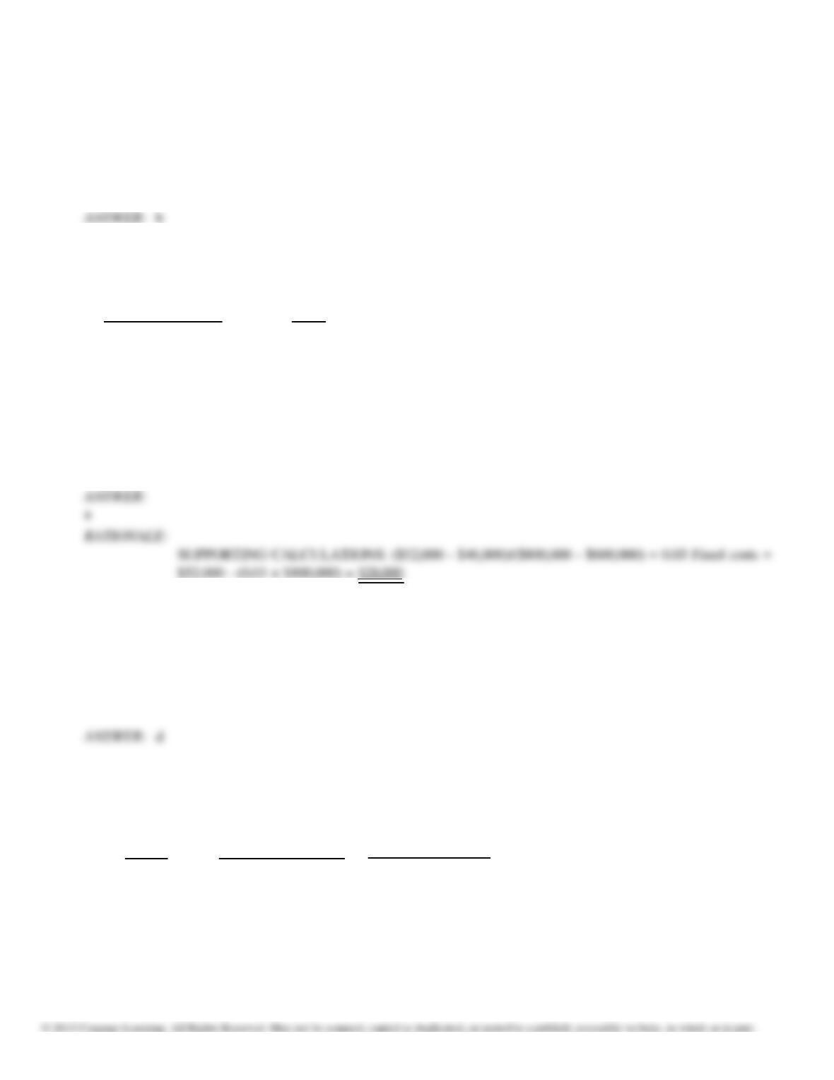
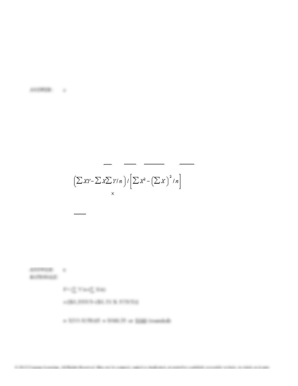
RATIONALE: SUPPORTING CALCULATIONS:
Month
X
y
XY
x2
June
75
$250
$18,750
5,625
July
115
310
35,650
13,225
August
190
400
76,000
36,100
September
60
240
14,400
3,600
October
135
355
47,925
18,225
Totals
575
1,555
$192,725
76,775
V=
= [$192,725 – (575 $1,555/5)]/[76,775 – (575)2/5]
= ($192,725 – $178,825)/(76,775 – 66,125)
= $13,900/10,650
= $1.31
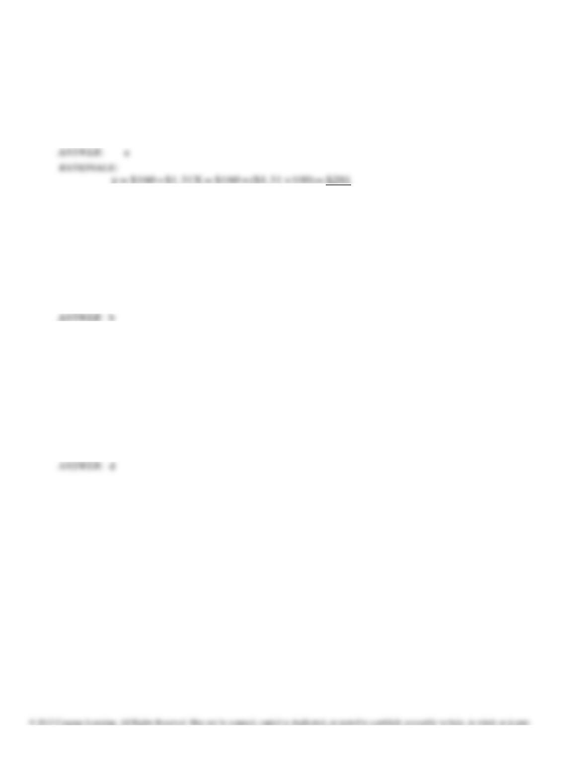
152.
Refer to Figure 3-6. Using a computer or calculator, compute the estimate of the fixed portion of
maintenance costs
using the method of least squares. Rounded to dollars, this value would be
a.
$575
b.
$166
c.
$160
d.
$66
Chapter 3: Cost Behavior
153.
Refer to Figure 3-6. Using a computer or calculator, compute the estimate of maintenance costs at
100 units of production using the method of least squares. This value would be
a. $291.
b. $321.
c. $336.
d. $698.
154.
The hypothesis test of cost parameters
a.
is not tested by the t-statistic.
b.
indicates whether the parameters are different from zero.
c.
tells the t-value of the significance achieved.
d.
all of the above.
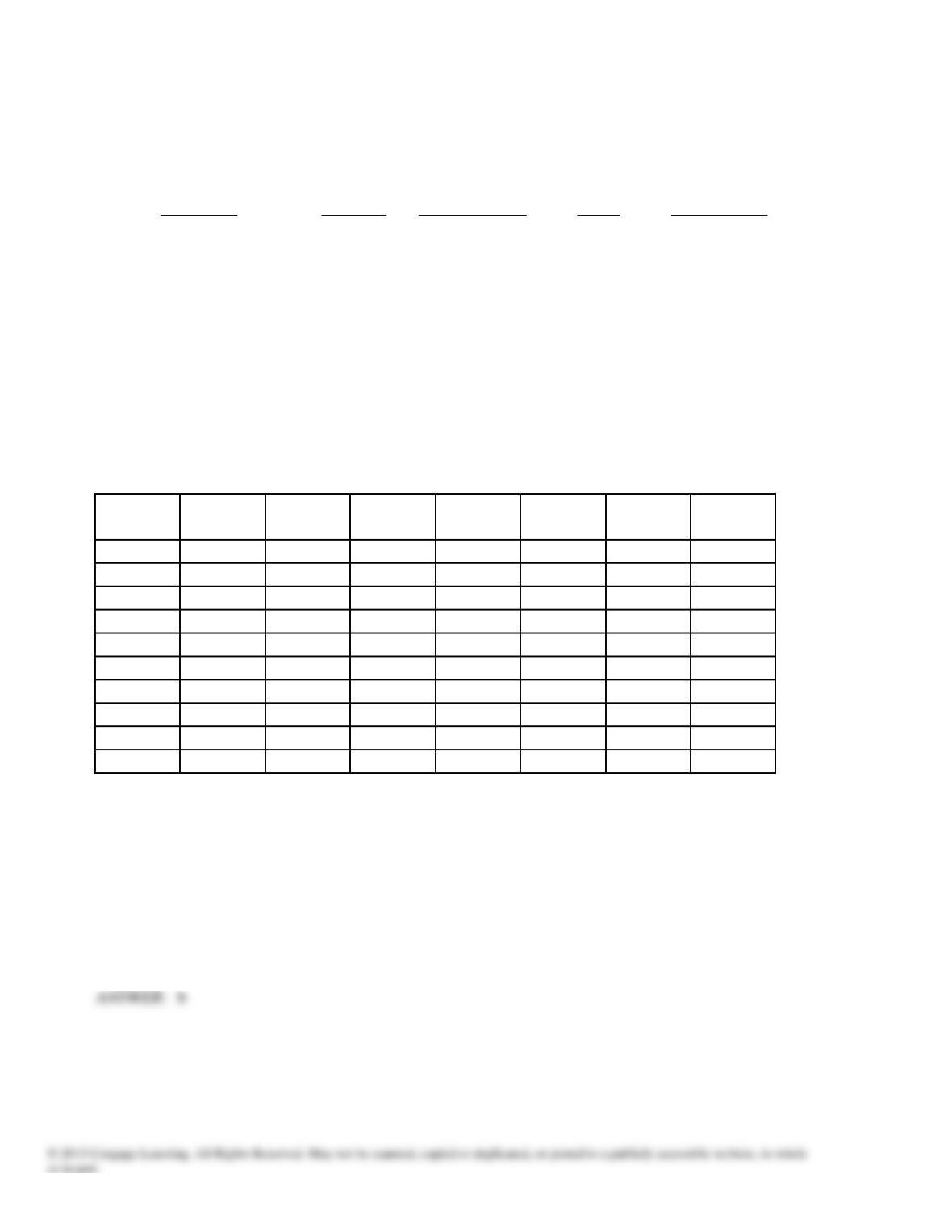
155.
The coefficient of determination is
a.
a measure of the variability of actual costs around the cost-estimating equation.
b.
used to construct probability intervals for cost estimates.
c.
a standardized measure of the degree to which two variables move together.
d.
a measure of the percent variation in the dependent variable that is explained by an independent
variable.
Chapter 3: Cost Behavior
Figure 3-7
The following computer printout estimated overhead costs using regression:
t for H(0)
Std. error
Parameter
Intercept
Estimate
100.41
Parameter = 0
4.81
Pr > t
0.0003
of parameter
20.88
DLH
14.05
6.78
0.0001
2.07
R Square (R2)
0.80
Standard Error (Se)
25.03
Observations
17
Please find the following statistical table
degrees
of freedom
90%
95%
99%
degrees of
freedom
90%
95%
99%
1
6.314
12.708
63.657
11
1.796
2.201
3.106
2
2.920
4.303
9.925
12
1.782
2.179
3.055
3
2.353
3.182
5.841
13
1.771
2.160
3.055
4
2.132
2.776
4.604
14
1.761
2.145
3.012
5
2.015
2.571
4.032
15
1.753
2.131
2.947
6
1.943
2.447
3.707
16
1.746
2.120
2.921
7
1.895
2.365
3.499
17
1.740
2.110
2.898
8
1.860
2.306
3.355
18
1.734
2.101
2.878
9
1.833
2.262
3.250
19
1.729
2.093
2.861
10
1.812
2.228
3.169
20
1.725
2.086
2.845
During the last accounting period 10,000 DLH were worked
.
156. Refer to Figure 3-7. What is the model?
a. Overhead = 4.81 + 6.78 DLH
b. Overhead = 100.41 + 14.05 DLH
c. Overhead = 14.05 + 100.41 DLH
d. DLH = 4.81 + 6.78 Overhead
Chapter 3: Cost Behavior
157. Refer to Figure 3-7. The coefficient of determination in this model tells us that
a. the slope is 14.05.
b. the intercept is 100.41.
c. 80 percent of the variation in the overhead variable is explained by DLH.
d. the slope is significant.
158. Refer to Figure 3-7. The hypothesis tests of the cost parameters indicate(s) that
a. the slope is significantly different from zero.
b. the intercept is significantly different from zero.
c. both the slope and intercept are not significant.
d. both the slope and intercept are significant.
159. Refer to Figure 3–7. Find the t-value for a 90 percent
confidence level. a. 1.740
b. 1.753
c. 6.314
d. 2.920
160. Refer to Figure 3-7. What is the confidence interval for the predicted overhead cost rounded to the
nearest whole number for a 90 percent confidence level?
a. predicted value between 140,557 and 140,644
b. predicted value between 140,644 and 140,731
c. predicted value between 87,000 and 130,500
d. none of these
161. A coefficient of determination of 0.91 means
a. the two variables move together in the same direction and have a strong relationship.
b. the parameter is not significant.
c. the model is significant 91 percent of the time.
d. that the independent variable explains 91 percent of the cost.

Chapter 3: Cost Behavior
162. What is the difference between a correlation equal to –1 and a correlation equal to 0?
a. A correlation equal to –1 means two alternatives are moving in the same direction, whereas a
correlation of 0 means they are moving in opposite directions.
b. A correlation equal to –1 means two alternatives are moving in the same direction, whereas a
correlation of 0 means they are unrelated.
c. A correlation equal to –1 means two alternatives are moving in opposite directions, whereas a
correlation of 0 means they are moving in the same direction.
d. A correlation equal to -1 means two alternatives are moving in opposite directions, whereas a
correlation of 0 means they are unrelated.
163. A managerial accountant has determined the following relationships between overhead and several
possible bases:
Basis
Correlation with Total
Overhead
Direct labor hours
0.842
Direct labor dollars
0.279
Machine hours
-0.837
Employee minutes in coffee breaks
-0.243
The best basis for overhead application is
a. direct labor hours.
b. coffee breaks.
c. direct labor dollars.
d. machine hours.
164. What is the difference between a correlation equal to –1 and a correlation equal to +1?
a. A correlation equal to –1 means two alternatives are moving in the same direction, whereas a
correlation of
+1 means they are moving in opposite directions.
b. A correlation equal to –1 means two alternatives are moving in the same direction, whereas a
correlation of
+1 means they are unrelated.
c. A correlation equal to –1 means two alternatives are moving in opposite directions, whereas a
correlation of
+1 means they are moving in the same direction.
d. A correlation equal to –1 means two alternatives are moving in opposite directions, whereas a
correlation of
+1 means they are unrelated.

Chapter 3: Cost Behavior
165. What does a correlation coefficient near +1 mean?
a. Two variables are moving in the opposite direction.
b. Two variables are moving in the same direction.
c. Two variables are unrelated.
d. One variable is not a good predictor of the other.
166. The appropriate range for the coefficient of
correlation (r) is
a. 0 ≤ r ≤ 1.
b. -% ≤ r ≤ +%.
c. –1 ≤ r ≤ 1.
d. –1 ≤ r ≤ +%.
167. What does a correlation coefficient near 0 mean?
a. Two variables are moving in the opposite direction.
b. Two variables are moving in the same direction.
c. Two variables are unrelated.
d. One variable is a good predictor of the other.
168. Which of the following statements is NOT true?
a. In selecting an independent variable for cost behavior analysis, it is important to determine the activity
that causes the cost being analyzed to occur.
b. Professional judgment is very important in selecting an activity measure for a particular cost.
c. A low correlation between two variables proves that one causes the other.
d. The least-squares cost estimation method can be used to measure the linear function.
169. What does a correlation coefficient near –1 mean?
a. Two variables are moving in the opposite direction.
b. Two variables are moving in the same direction.
c. Two variables are unrelated.
d. One variable is not a good predictor of the other.
Chapter 3: Cost Behavior
90%
95%
99%
1.753
2.131
2.947
1.746
2.120
2.921
1.740
2.110
2.898
1.734
2.101
2.878
1.729
2.093
2.861
170. The confidence interval for the predicted value of Y
a. is a measure of the likelihood that the prediction interval will not contain the actual cost.
b. is constructed by multiplying the t-statistic times the standard error.
c. can only be computed with 95 percent confidence.
d. all of the above.
171. The following data is available of estimated overhead costs using linear regression:
t for H(0)
Std. error
Intercept
Parameter
Estimate
100.41
Parameter = 0
4.81
Pr > t
0.0003
of parameter
20.88
DLH
14.05
6.78
0.0001
2.07
R Square (R 2)
0.80
Standard Error (Se)
25.03
Observations
17
Table of Selected Values: t Distribution
Degrees of
Freedom
15
16
17
18
19
What is the interval around Y if 95 percent confidence is desired?
a. Y ± 20.024
b. Y ± 43.87759
c. Y ± 52.8133
d. Y ± 53.33893

Chapter 3: Cost Behavior
Figure 3-8
The following computer printout estimated overhead costs using multiple regression:
t for H(0)
Std. error
Intercept
Parameter
Estimate
1000
Parameter = 0
1.96
Pr > t
0.0250
of parameter
510.204
Setup hours
25
81.96
0.0001
0.305
# of parts
100
9.50
0.0001
10.527
R Square (R2)
0.94
Standard Error (Se)
75.00
Observations
160
During the year the company used 1,000 setup hours and 500 parts.
172. Refer to Figure 3-8. The degrees of freedom for the model is
a. 158
b. 157
c. 159
d. 160
173. Refer to Figure 3-8. Which slope and intercept parameters are significant at the 0.05 level?
a. intercept
b. setup hours
c. number of parts
d. all of the above
174. Refer to Figure 3-8. The model being measured is
a. Overhead = 1,000 + 25(Setup hours) + 100(# of parts)
b. Overhead = 510 + 0.305(Setup hours) + 10.527(# of parts)
c. Overhead = 0.98 + 40.98(Setup hours) + 4.865(# of parts)
d. Overhead = 1,000 + 25(Setup hours)