212)
As a firm increases the level of output that it produces, short–run average fixed cost
212)
A)
decreases up to a particular level of output and then increases.
B)
decreases.
C)
rises and then falls.
D)
remains constant since fixed costs are constant.
213)
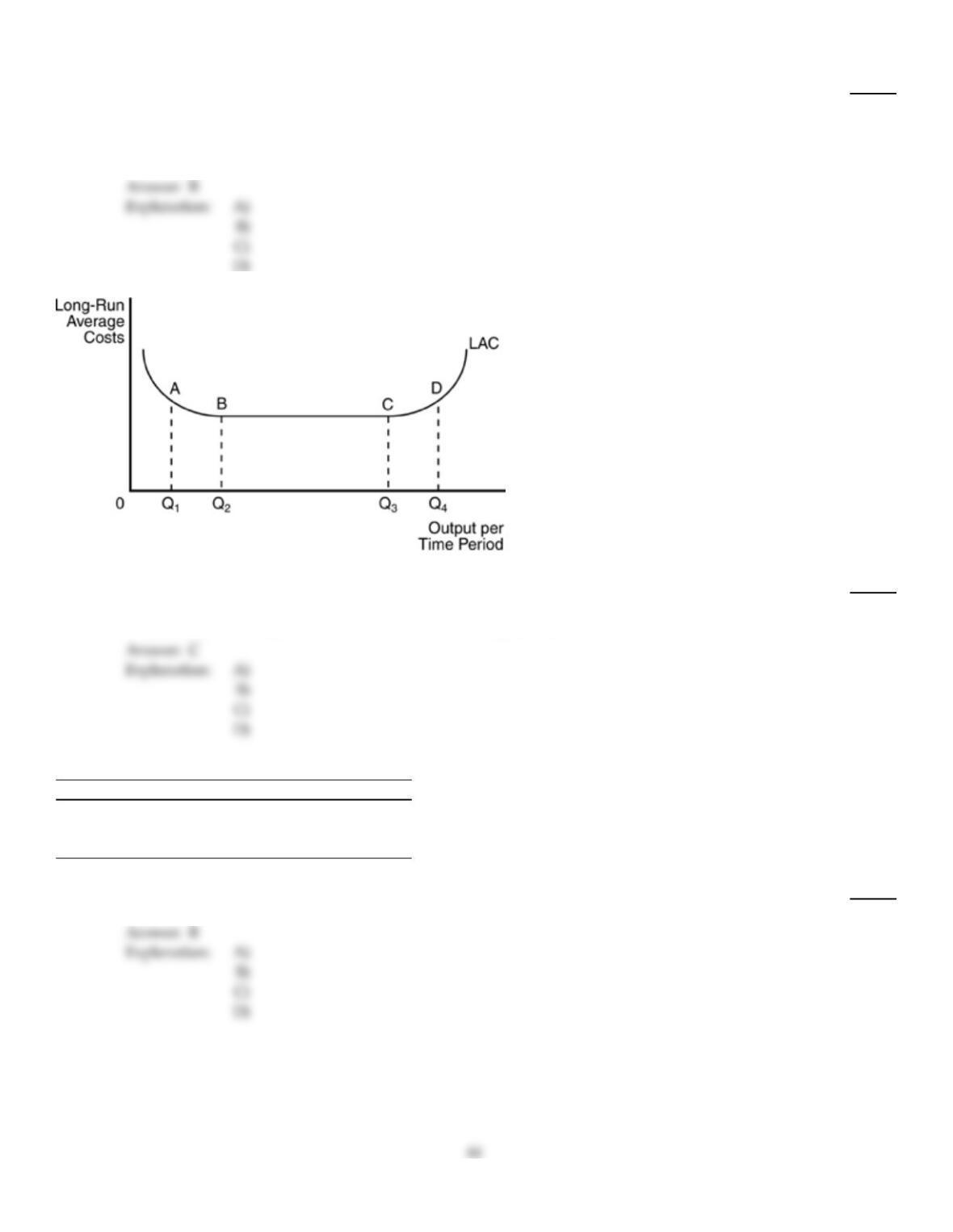
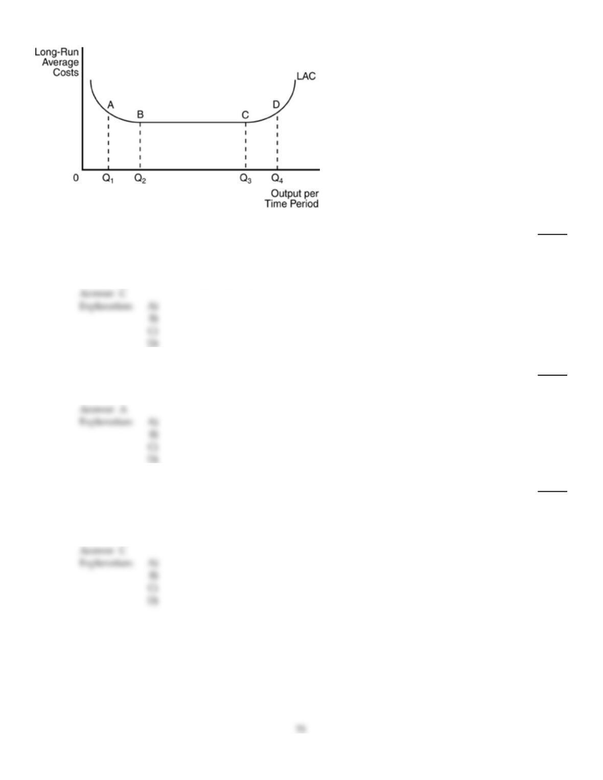
In the above figure, for any output level less than Q2, this firm experiences
213)
A)
constant economies of scale.
B)
decreasing long run average costs.
C)
economies of scale.
D)
diseconomies of scale.
QTFC TVC TC AFC AVC ATC
1
2$75 $25
3$40
214)
Refer to the above table. What are total variable costs at an output of 2 units?
214)
A)
$100
B)
$50
C)
$200
D)
$150
215)
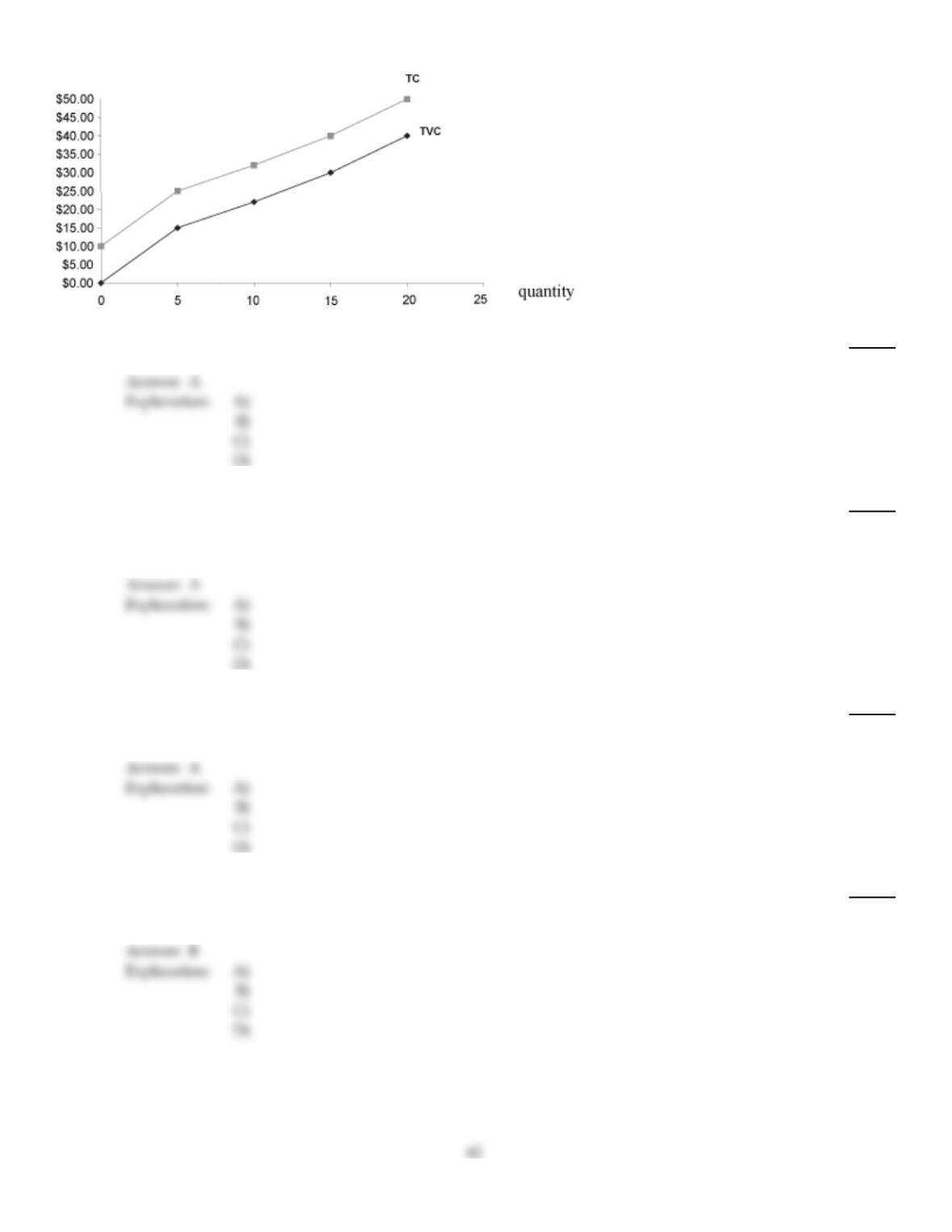
Use the above figure. The AVC at output 5 is
215)
A)
$3.00.
B)
$5.00.
C)
$2.00.
D)
$35.00.
216)
Phil found that as he continued to crowd laborers into his hot dog stand, the extra output he was
receiving from each additional laborer was beginning to fall off. This is an example of the
216)
A)
law of diminishing product.
B)
law of demand.
C)
law of diminishing marginal utility.
D)
law of increasing opportunities.
217)
The typical cost curves are U–shaped due to the
217)
A)
law of diminishing marginal product.
B)
law of demand.
C)
law of supply.
D)
law of diminishing marginal utility.
218)
The time period during which all factors of production can be varied is the
218)
A)
production time.
B)
long run.
C)
calendar year.
D)
short run.
219)
Which of the following statements about a firm‘s short–run variable costs is correct?
219)
A)
They increase as the level of output decreases.
B)
They are always a greater expense than are fixed costs.
C)
They typically include the cost of workers’ wages.
D)
They include the costs of plant and equipment.
220)
The physical output that is due to the addition of one more unit of a variable factor of production is
220)
A)
average product.
B)
average total cost.
C)
marginal cost.
D)
marginal product.
221)
Diseconomies to scale are illustrated by
221)
A)
a downward sloping long–run average cost curve.
B)
a horizontal long–run average cost curve.
C)
an upward sloping long–run average cost curve.
D)
a long–run average cost curve that is shaped like an upside down U.
222)
Production functions indicate the relationship between
222)
A)
factor costs and output prices.
B)
factor inputs and factor prices.
C)
factor inputs and the quantity of output.
D)
the value of inputs and average costs.
223)
If the price of labor is constant and a firm experiences diminishing marginal product, then its
223)
A)
average variable cost increases.
B)
fixed costs increase.
C)
total costs decrease.
D)
marginal costs decrease.
224)
The typical shape of the long–run average cost curve is like
224)
A)
the letter “U.“
B)
the letter “C.”
C)
an inverse of the letter “V.”
D)
a circle.
Total Output Total Costs
0 $10
1 18
2 21
3 23
4 24
5 26
6 29
7 33
8 38
9 44
10 51
225)
Using the above table, we see that when output is 4 units, average variable cost equals
225)
A)
$14.00.
B)
$6.00.
C)
$24.00.
D)
$3.50.
226)
The relationship Q = f(K, L) is an example of a
226)
A)
profit equation.
B)
production function.
C)
demand equation.
D)
cost function.
Total Output Total Costs
0 $10
1 18
2 21
3 23
4 24
5 26
6 29
7 33
8 38
9 44
10 51
227)
In the above table, when output is 8 units, average variable costs are
227)
A)
$4.50.
B)
$3.50.
C)
$1.25.
D)
$4.75.
228)
The total cost of the firm
228)
A)
includes explicit costs but excludes implicit costs.
B)
includes implicit and explicit costs.
C)
includes implicit costs but excludes explicit costs.
D)
includes implicit and explicit costs but excludes a normal rate of return on investment.
229)
Suppose that one worker can produce 15 cookies, two workers can produce 35 cookies together,
and three workers can produce 60 cookies together. What is the average product of the first three
workers?
229)
A)
17.5 cookies
B)
30 cookies
C)
20 cookies
D)
25 cookies
230)
When the average physical product is falling
230)
A)
average variable costs are falling.
B)
average fixed costs are rising.
C)
average variable costs are rising.
D)
total costs are falling.
QTFC TVC TC
0$90 $ 0 $ 90
190 25 115
290 32 122
390 42 132
490 64 154
590 95 185
231)
Refer to the above table. What is AVC at an output of 2 units?
231)
A)
$7
B)
$45
C)
$16
D)
$61
Use the information from the below table to answer following question(s).
Input of Total
Labor Product
0 0
120
2 50
380
4105
5125
6140
7150
232)
In the above table, the average product for 5 units of labor is
232)
A)
15.0.
B)
20.0.
C)
22.5.
D)
25.0.
D
233)
Which of the following would be a fixed input for an amusement park?
233)
A)
ticket takers
B)
concession workers
C)
unpopped popcorn
D)
the roller coaster
D
C
234)
Which of the following is NOT correct?
234)
A)
ATC = TC/Q
B)
MC = change in TC/change in Q
C)
ATC + AVC = AFC
D)
AVC = TVC/Q
Total Output Total Costs
0 $10
1 18
2 21
3 23
4 24
5 26
6 29
7 33
8 38
9 44
10 51
235)
Using the above table, we see that when output is 4 units, average total cost equals
235)
A)
$14.00.
B)
$3.50.
C)
$24.00.
D)
$6.00.
Quantity of Total Average Marginal
Workers Product Product Product
0 0
1 3
2 7
312
416
518
618
236)
In the above table, the marginal physical product of the 6th worker is
236)
A)
0.
B)
3.
C)
5.
D)
4.
237)
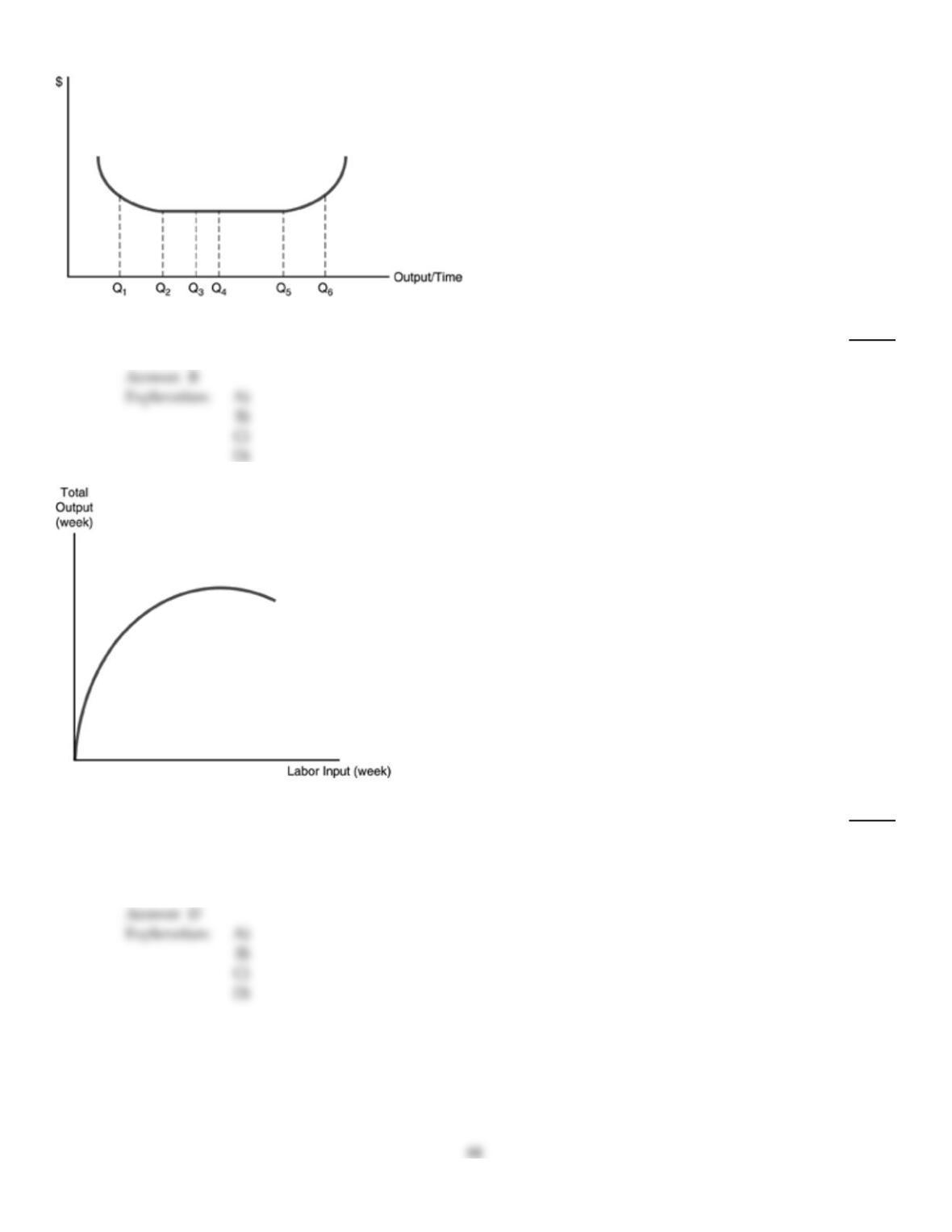
Refer to the above figure. Minimum efficient scale is at output rate
237)
A)
Q1.
B)
Q2.
C)
Q3.
D)
Q5.
238)
Refer to the above figure. The curve reflects
238)
A)
the law of increasing marginal product in capital.
B)
the law of diminishing marginal product in capital.
C)
the law of increasing marginal product in labor.
D)
the law of diminishing marginal product in labor.
Fixed Variable Total Average Average Marginal
Output Costs Costs Costs Total Costs Variable Costs Costs
0$0 $100
130
250
3 60
4 120
5200
239)
In the above table, what are the total fixed costs for an output of 4?
239)
A)
$100
B)
$0
C)
$120
D)
$220
240)
Marginal costs will begin to rise at the point where
240)
A)
diminishing marginal product begins.
B)
average variable costs increase.
C)
variable costs increase.
D)
fixed costs increase.
Fixed Variable Total Average Average Marginal
Output Costs Costs Costs Total Costs Variable Costs Costs
0$0 $100
130
250
3 60
4 120
5200
241)
In the above table, what is the average variable cost to produce 2 units of output?
241)
A)
$55
B)
$20
C)
$60
D)
$30
242)
Average variable cost equals
242)
A)
TC/Q.
B)
TVC/Q.
C)
TFC/Q.
D)
change in total cost/change in output.
243)
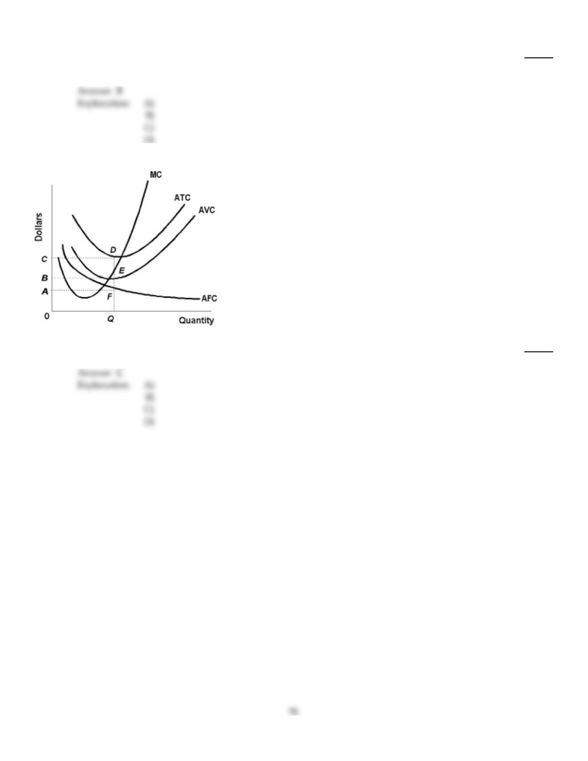
Use the above figure. At an output equal to “Q” the total variable cost for the firm will be the area
243)
A)
OQFA.
B)
OQAB.
C)
OQEB.
D)
OQDC.
244)
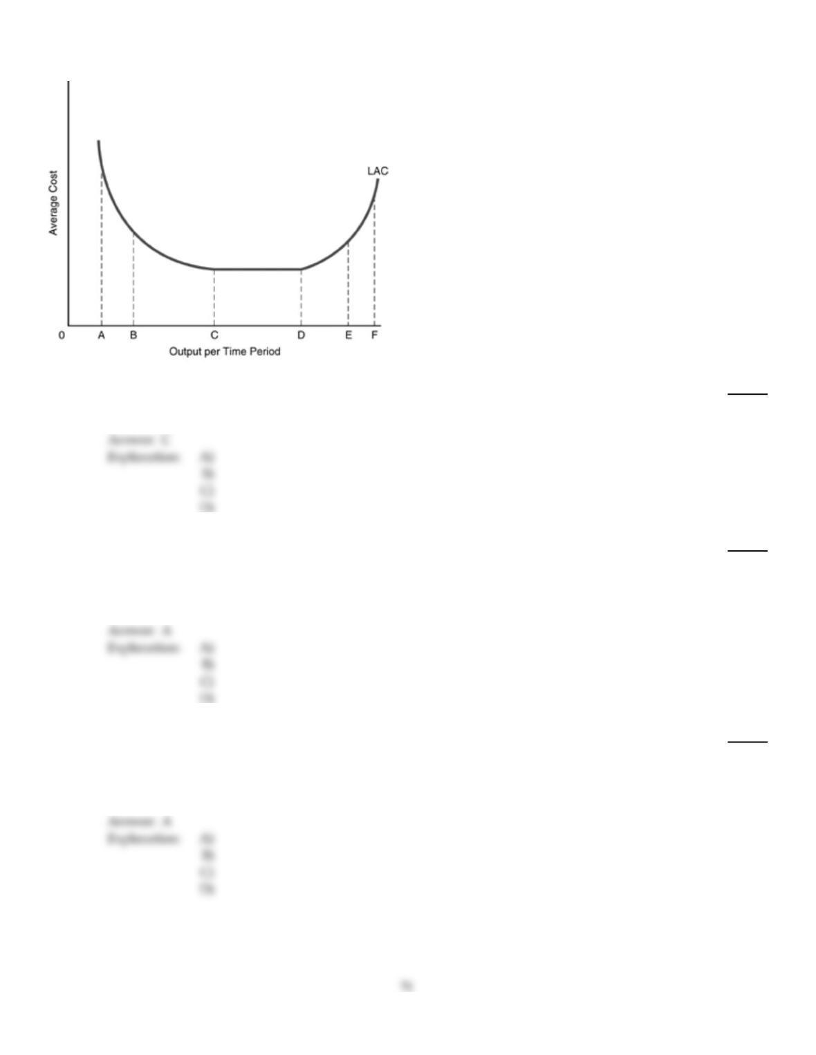
In the above figure, the long–run cost curve between points C and D illustrates
244)
A)
diseconomies of scale.
B)
diminishing marginal product.
C)
constant returns to scale.
D)
economies of scale.
245)
Total product will start to decrease
245)
A)
when marginal physical product becomes negative.
B)
when average physical product decreases.
C)
when marginal physical product increases.
D)
at the quantity where the law of diminishing returns starts.
246)
Economies to scale are illustrated by
246)
A)
a downward sloping long–run average cost curve.
B)
a horizontal long–run average cost curve.
C)
an upward sloping long–run average cost curve.
D)
a long–run average cost curve that is shaped like an upside down U.
247)
A fixed resource is one that
247)
A)
cannot be varied in the short run.
B)
costs more than the average daily revenue of the firm.
C)
can be disposed of only if the firm goes out of business.
D)
is physically tied to a specific location.
248)
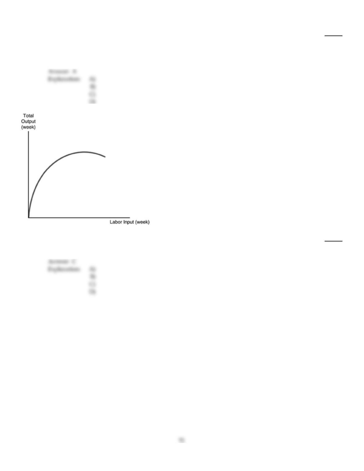
Refer to the above figure. The curve represents a
248)
A)
average total cost curve.
B)
marginal product curve.
C)
total product curve.
D)
total cost curve.
249)
In the above figure, point B is called
249)
A)
the planning horizon.
B)
the maximum efficient scale.
C)
the minimum efficient scale.
D)
the point of diminishing marginal product.
250)
For a hotdog vendor, the hotdog buns represents his
250)
A)
variable input.
B)
sunk cost.
C)
fixed input.
D)
none of the above.
A
251)
Minimum efficient scale is defined as
251)
A)
the amount of labor that maximizes the marginal product of labor.
B)
the point at which marginal cost, average variable cost, and average fixed cost are all equal.
C)
the lowest output level at which long–run average costs are at their minimum.
D)
the point at which economies of scale are at their maximum.
C
C
252)
Short–run cost relationships for a firm are
252)
A)
determined by the specific long–run relationships that exist.
B)
due to the normal contractual relations in a market.
C)
determined by the law of diminishing marginal product.
D)
due to the level of wages relative to other input prices.
253)
If the average product of 20 workers is 100 bushels of wheat and the average product of 21 workers
of wheat is 99 bushels of wheat, then the marginal product of the 21st worker was
253)
A)
5 bushels of wheat.
B)
79 bushels of wheat.
C)
–1 bushel of wheat.
D)
99 bushels of wheat.
Explanation:
254)
The planning curve is the
254)
A)
short–run marginal cost curve.
B)
long–run average cost curve.
C)
short–run average cost curve.
D)
production function.
Explanation:
255)
Notice the costs as given in the table below. What is the marginal cost when total cost is $23?
Total Output Total Costs
0 $10
1 $15
2 $18
3 $20
4 $21
5 $23
255)
A)
$2
B)
$5
C)
$3
D)
$1
Explanation:
Explanation:
256)
Which of the following is correct?
256)
A)
TC = AVC
Q
B)
MC = TC – TVC
C)
AFC = TC/Q – TVC/Q
D)
AVC = TVC – AFC
257)
When increasing its output results in falling costs, a firm that can adjust all inputs is experiencing
257)
A)
economies of scale.
B)
diseconomies of scale.
C)
capital gains.
D)
loss.
A
258)
In the short run, average total cost is
258)
A)
less than average variable cost.
B)
sometimes higher and sometimes lower than average variable cost.
C)
higher than average variable cost.
D)
equal to average variable cost.
C
259)
Suppose the manager of a restaurant notices that when she has too many waiters on the floor for a
shift that the waiters get in each other’s way and fewer dinners are served. This is an example of
259)
A)
diminishing marginal workforce.
B)
diminishing marginal product.
C)
diminishing marginal inputs.
D)
diminishing marginal utility.
B
260)
The long–run average cost curve
260)
A)
is always a downward sloping straight line.
B)
should always be horizontal.
C)
is identical to the marginal cost curve.
D)
is a curve which is tangent to each member of a set of short–run average cost curves.
D
C
261)
The law of diminishing marginal product is NOT responsible for the shape of
261)
A)
marginal cost curve.
B)
the total cost curve.
C)
the average variable cost curve.
D)
total fixed cost curve.
262)
Marginal cost is equal to
262)
A)
change in total variable cost divided by change in output.
B)
change in total cost divided by change in output.
C)
total variable cost divided by quantity of output.
D)
Both A and B are correct.
Fixed Variable Total Average Average Marginal
Output Costs Costs Costs Total Costs Variable Costs Costs
0$0 $100
130
250
3 60
4 120
5200
263)
In the above table, what is the marginal cost to produce the 2nd unit of output?
263)
A)
$20
B)
$60
C)
$30
D)
$55
264)
Constant returns to scale are illustrated by
264)
A)
a downward sloping long–run average cost curve.
B)
a horizontal long–run average cost curve.
C)
an upward sloping long–run average cost curve.
D)
a long–run average cost curve that is shaped like an upside down U.
Total Output Total Costs
0 $10
1 18
2 21
3 23
4 24
5 26
6 29
7 33
8 38
9 44
10 51
265)
In the above table, total fixed costs are
265)
A)
$18.00.
B)
$5.00.
C)
$10.00.
D)
$8.00.
QTFC TVC TC AFC AVC ATC
1
2$75 $25
3$40
266)
Refer to the above table. What are total costs at an output of 3 units?
266)
A)
$120
B)
$150
C)
$270
D)
$90
267)
Which one of the following statements is FALSE?
267)
A)
MC = TC divided by Q
B)
ATC = AFC + AVC
C)
AFC = TFC divided by Q
D)
TC = TFC + TVC
268)
Suppose that one worker can produce 15 cookies, two workers can produce 35 cookies together,
and three workers can produce 60 cookies together. What is the marginal product of the 3rd
worker?
268)
A)
60 cookies
B)
25 cookies
C)
35 cookies
D)
20 cookies
269)
The addition to total costs associated with the production of one more unit of output is referred to
as
269)
A)
opportunity cost.
B)
average cost.
C)
marginal cost.
D)
overhead cost.
270)
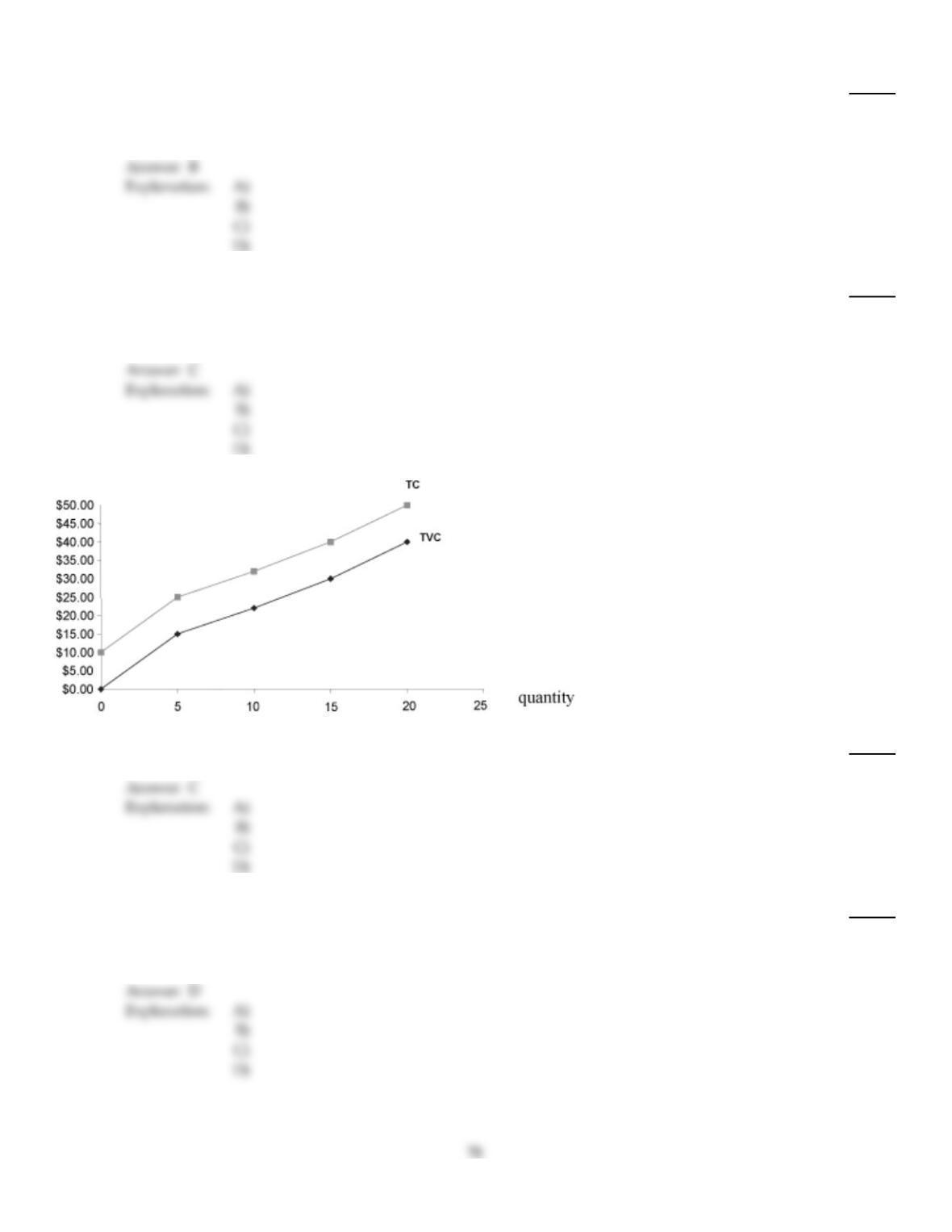
Use the above figure. The AFC at output level 20 is
270)
A)
$10.00.
B)
$3.00.
C)
$0.50.
D)
$1.00.
271)
The change in total product occurring when a variable input is increased and all other inputs are
held constant is
271)
A)
marginal cost.
B)
average total cost.
C)
average product.
D)
marginal product.
272)
The point of saturation occurs when a firm
272)
A)
first experiences positive marginal product.
B)
maximizes its total returns.
C)
first encounters negative marginal product.
D)
has total returns equal to zero.
273)
Which of the following is TRUE?
273)
A)
If MC is below AVC, AVC must be increasing.
B)
If MC is above ATC, ATC must be increasing.
C)
The MC curve intersects AFC at its minimum point.
D)
none of the above
B
274)
As a firm continues to produce additional output, which of the following will continue to decline as
output expands?
274)
A)
average total costs
B)
average fixed costs
C)
opportunity costs
D)
marginal costs
B
275)
The change in output caused by a one–unit change in labor is referred to as the
275)
A)
compounded physical product of labor.
B)
total product of labor.
C)
marginal product of labor.
D)
average product of labor.
C
276)
The marginal productivity of labor will eventually decrease as more workers are employed because
276)
A)
the amount of capital will also be increasing.
B)
on the average each worker will have fewer inputs to work with.
C)
average product is increasing.
D)
total product is decreasing.
B
C
Use the information from the below table to answer following question(s).
Input of Total
Labor Product
0 0
120
2 50
380
4105
5125
6140
7150
277)
In the above table, the marginal product of the fourth worker is
277)
A)
20.
B)
30.
C)
25.
D)
15.
278)
Suppose a firm doubles its output in the long run. At the same time the unit cost of production
remains unchanged. We can conclude that the firm is
278)
A)
not using the available technology efficiently.
B)
exploiting the economies of scale available to it.
C)
facing constant returns to scale.
D)
facing diseconomies of scale.
Average
Labor Output Product Marginal Product
110 –
212
315
4 52
5 9
279)
Using the above table, the marginal product of the 4th worker is
279)
A)
13.
B)
14.
C)
12.
D)
15.