The Theory of Consumer Choice 5359
8. Refer to Figure 21-30. Suppose Budget Constraint B applies. If the consumer’s income is $90
and if he is buying 5 light bulbs, then how much money is he spending on hamburgers?
9. If the market is offering consumers the trade-off of 3 pints of Pepsi for 1 pizza, and if the price of a
pizza is $9, then what is the price of a pint of Pepsi?
10. A consumer’s budget constraint is drawn with the quantity of pizza measured along the horizontal
axis and the price of Pepsi measured along the vertical axis. If the market is offering the
consumer the trade-off of 3 pints of Pepsi for 1 pizza, then what is the slope of the consumer’s
budget constraint?
5360 The Theory of Consumer Choice
11. What does the slope of a budget constraint represent?
12. A consumer’s budget constraint is drawn on a graph with the number of sandwiches measured
along the horizontal axis and the number of bowls of soup measured along the vertical axis. Hold
the consumer’s income and the price of a sandwich fixed, and increase the price of a bowl of
soup. Describe the effect on the budget constraint.
13. The rate at which a consumer is willing to trade off one good for another is called the .
The Theory of Consumer Choice 5361
14. In order to represent a consumer’s choices on a graph, we draw her budget constraint as well as
her curves.
15. When we draw Katie’s indifference curves to represent her preferences for books and movies,
we find that her indifference curves are upward-sloping. What does this tell us about Katie’s
preferences?
16. A consumer’s indifference curves are right angles when, for the consumer, the goods in question
are .
5362 The Theory of Consumer Choice
17. A consumer’s indifference curves are straight lines when, for the consumer, the goods in
question are__________________________.
18. What does the slope of a consumer’s indifference curve represent?
19. Because people are more willing to trade away goods that they have in abundance and less
willing to trade away goods of which they have little, indifference curves are ___________.
The Theory of Consumer Choice 5363
20. Teresa faces prices of $6.00 for a unit of good X and $1.50 for a unit of good Y. At her optimum,
Teresa is willing to give up 1 unit of good X for units of good Y.
21. Thomas faces prices of $6 for a unit of good X and $30 for a unit of good Y. At his optimum,
Thomas is willing to give up 1 unit of good Y for units of good X.
22. If goods X and Y are both normal goods for Brenda, then an increase in Brenda’s income will
lead her to__________.
5364 The Theory of Consumer Choice
23. Using our model of consumer choice, is it possible for a consumer to buy less of a particular good
when his income rises? Briefly explain.
24. What is significant about a point on a graph at which an indifference curve is tangent to a budget
constraint?
25. Goods x and y are available to Jeff. At Jeff’s optimum, the marginal utility per dollar spent on
good x equals__________________.
The Theory of Consumer Choice 5365
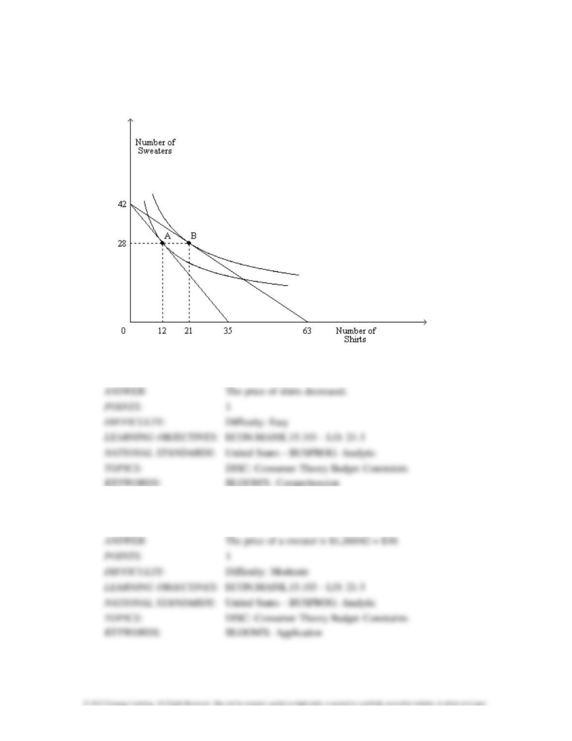
Figure 21-31
The figure shows two indifference curves and two budget constraints for a consumer named
Kevin.
26. Refer to Figure 21-31. Suppose point A was Kevin’s optimum last week, and point B is his
optimum this week. What happened between last week and this week?
27. Refer to Figure 21–31. If Kevin’s income is $1,260, then what is the price of a sweater?
5366 The Theory of Consumer Choice
28. Refer to Figure 21-31. If point A is Kevin’s optimum, then at that optimum, what is his
opportunity cost of a shirt in terms of sweaters?
29. Refer to Figure 21-31. If the price of a shirt is $36 and point A is Kevin’s optimum, then what
is Kevin’s income?
30. Refer to Figure 21-31. If Kevin’s income is $1,260 and point A is his optimum, then what is the
price of a shirt?
The Theory of Consumer Choice 5367
31. Refer to Figure 21-31. Suppose Kevin is optimally purchasing 12 shirts and 28 sweaters, and he
is spending $648 on shirts. What is the price of a sweater?
32. Refer to Figure 21-31. Suppose Kevin is optimally purchasing 21 shirts and 28 sweaters, and he
is spending $1,680 on sweaters. What is the price of a shirt?
33. Refer to Figure 21-31. If point B is Kevin’s optimum, then at that optimum, what is his
opportunity cost of a sweater in terms of shirts?
5368 The Theory of Consumer Choice
34. Refer to Figure 21-31. If the price of a shirt is $20 and point B is Kevin’s optimum, then what
is Kevin’s income?
35. Refer to Figure 21-31. If Kevin’s income is $2,520 and point B is his optimum, then what is the
price of a shirt?
36. Refer to Figure 21–31. For Kevin, are sweaters and shirts substitutes, complements, or neither?
The Theory of Consumer Choice 5369
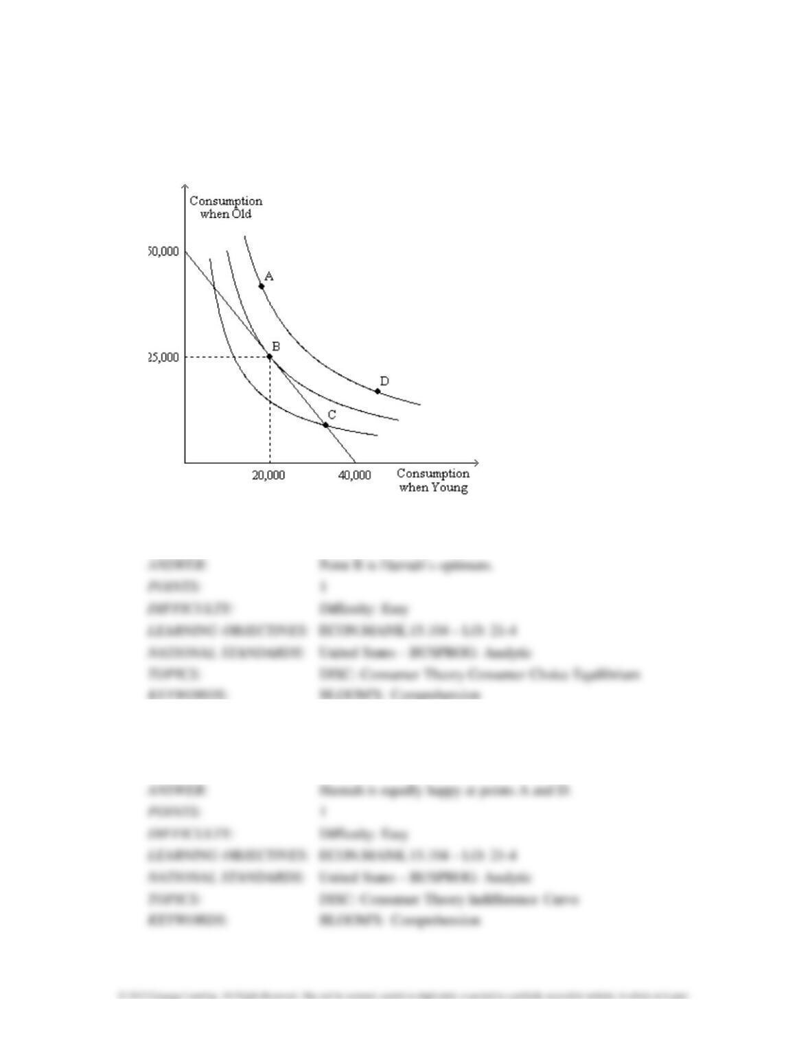
Figure 21-32
The figure shows three indifference curves and a budget constraint for a consumer named
Hannah. When young, Hannah works and earns income. When old, she is retired and earns no
income.
37. Refer to Figure 21-32. Which of the four labeled points is Hannah’s optimum?
38. Refer to Figure 21-32. At two of the four labeled points, Hannah is equally happy. Identify
those two points.

5370 The Theory of Consumer Choice
39. Refer to Figure 21-32. Of the four labeled points, which is (are) affordable to Hannah?
40. Refer to Figure 21-32. How much income does Hannah earn when she is young?
41. Refer to Figure 21-32. What is the value of the interest rate that Hannah earns on her saving?
The Theory of Consumer Choice 5371
42. Refer to Figure 21-32. If Hannah chose to spend $30,000 on consumption when young, then
how much could she spend on consumption when old?
43. Refer to Figure 21-32. From the figure we can determine how much income Hannah earns
when young and we can determine the interest rate. Could the interest rate rise to a level at
which Hannah could afford to be at point A?
44. Refer to Figure 21-32. From the figure we can determine how much income Hannah earns
when young and we can determine the interest rate. Could the interest rate rise to a level at
which Hannah could afford to be at point D?
45. Is it possible for a normal good to be a Giffen good? Briefly explain.
5372 The Theory of Consumer Choice
46. A field experiment conducted by economists in the Chinese province of Hunan provided evidence
that, for poor households in that province, rice is a good.
47. For Meg, the substitution effect of an interest-rate increase is stronger than the income effect. In
response to a higher interest rate, will Meg save more or will she save less?
The Theory of Consumer Choice 5373
48. For Molly, the substitution effect of a wage increase is stronger than the income effect. In
response to a wage increase, will Sally work more hours or will she work fewer hours?
49. For Brent, the income effect of a wage increase is stronger than the substitution effect. In
response to a wage increase, will Brent work more hours or will he work fewer hours?
50. For Antonio, the income effect of an interest-rate increase is stronger than the substitution effect.
In response to a higher interest rate, will Antonio save more or will he save less?