Chapter 19: Time Series Analysis – Quiz A Name _________________________
19.2.2 Identify components of time series.
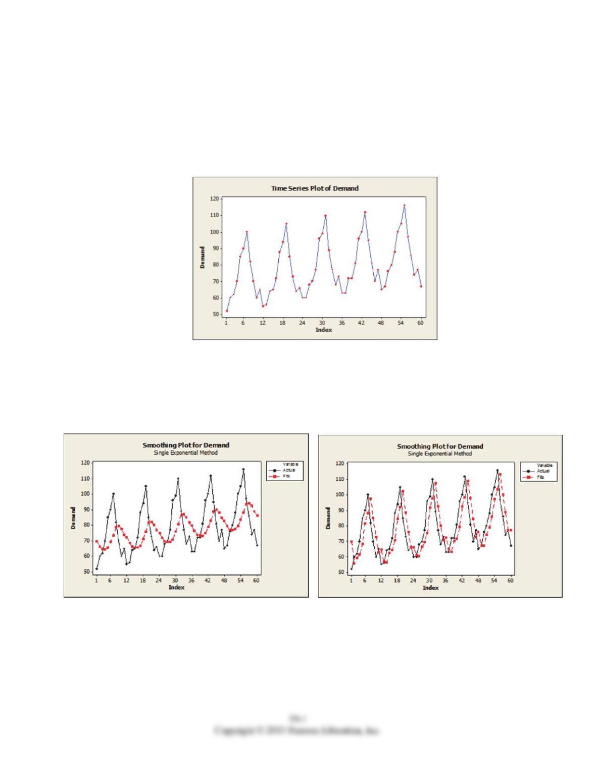
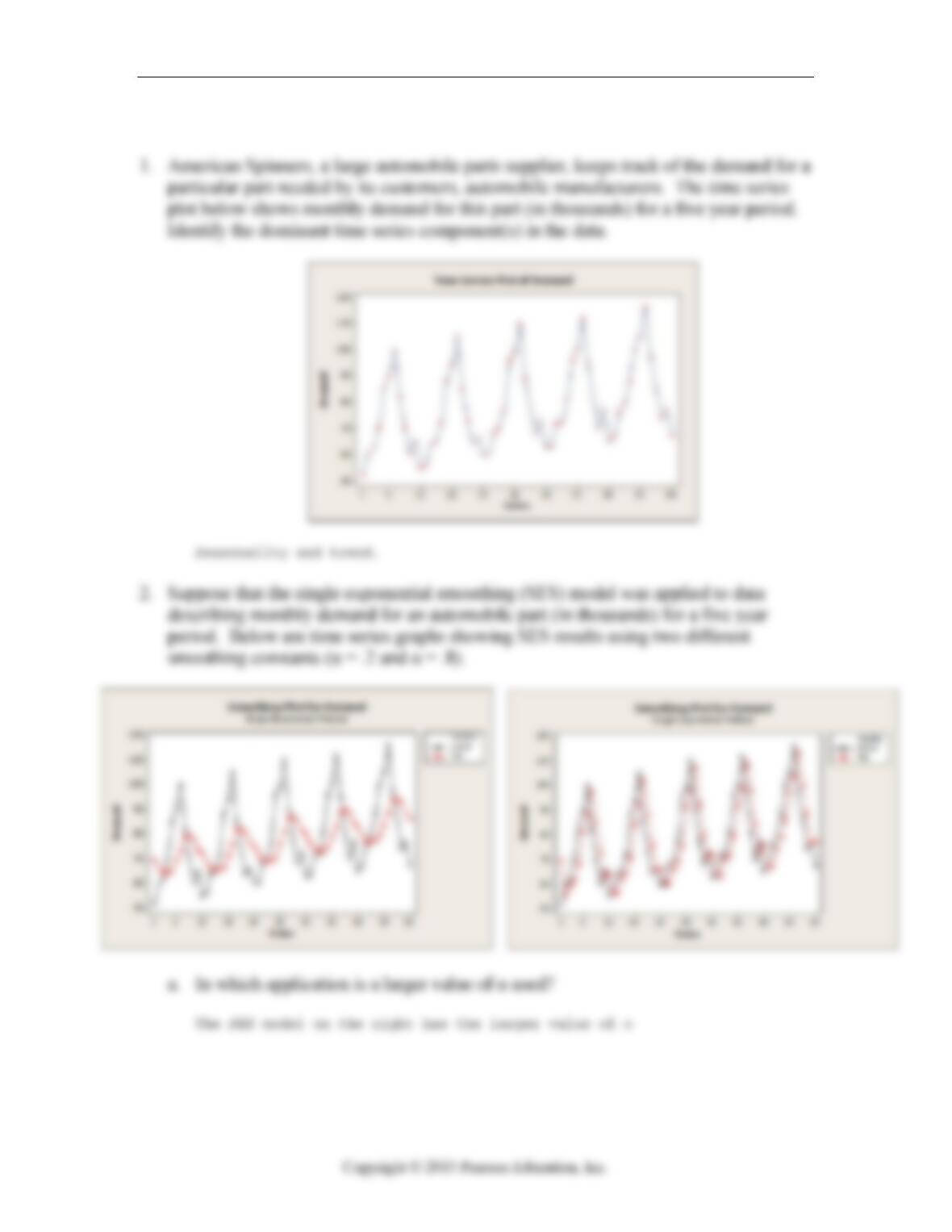
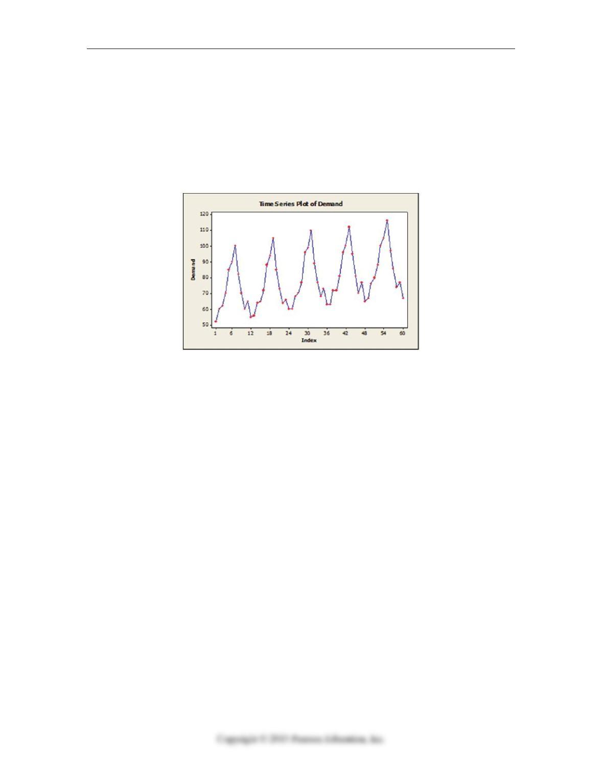
1. American Spinners, a large automobile parts supplier, keeps track of the demand for a
particular part needed by its customers, automobile manufacturers. The time series
plot below shows monthly demand for this part (in thousands) for a five year period.
Identify the dominant time series component(s) in the data.
19.3.4 Smooth time series models.
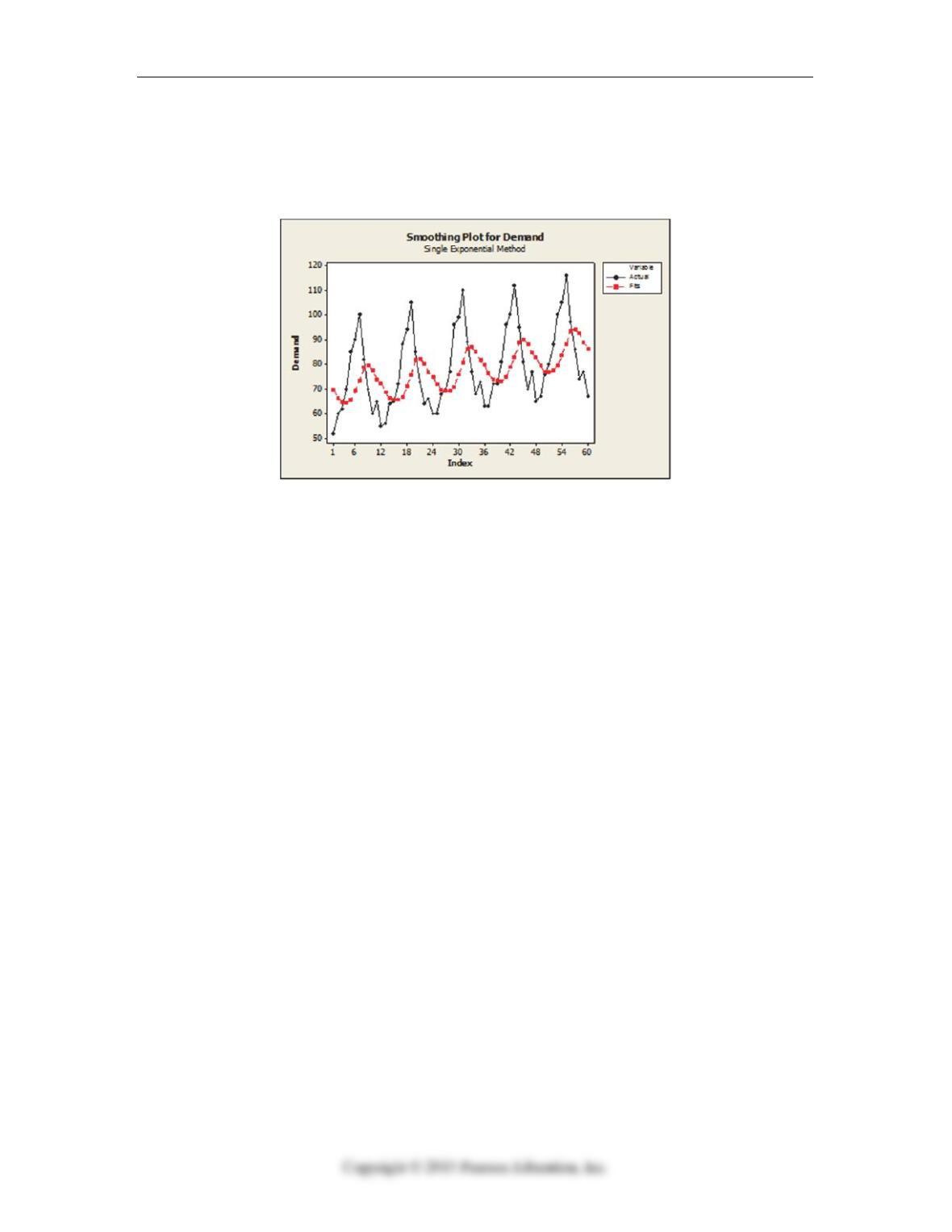
2. Suppose that the single exponential smoothing (SES) model was applied to data
describing monthly demand for an automobile part (in thousands) for a five year
period. Below are time series graphs showing SES results using two different
smoothing constants (α = .2 and α = .8).
a. In which application is a larger value of α used?
b. What forecasting method may be a better choice than SES for these data?
Explain.
19-2 Chapter 19 Time Series Analysis
19.7.8 Choose a forecasting method.
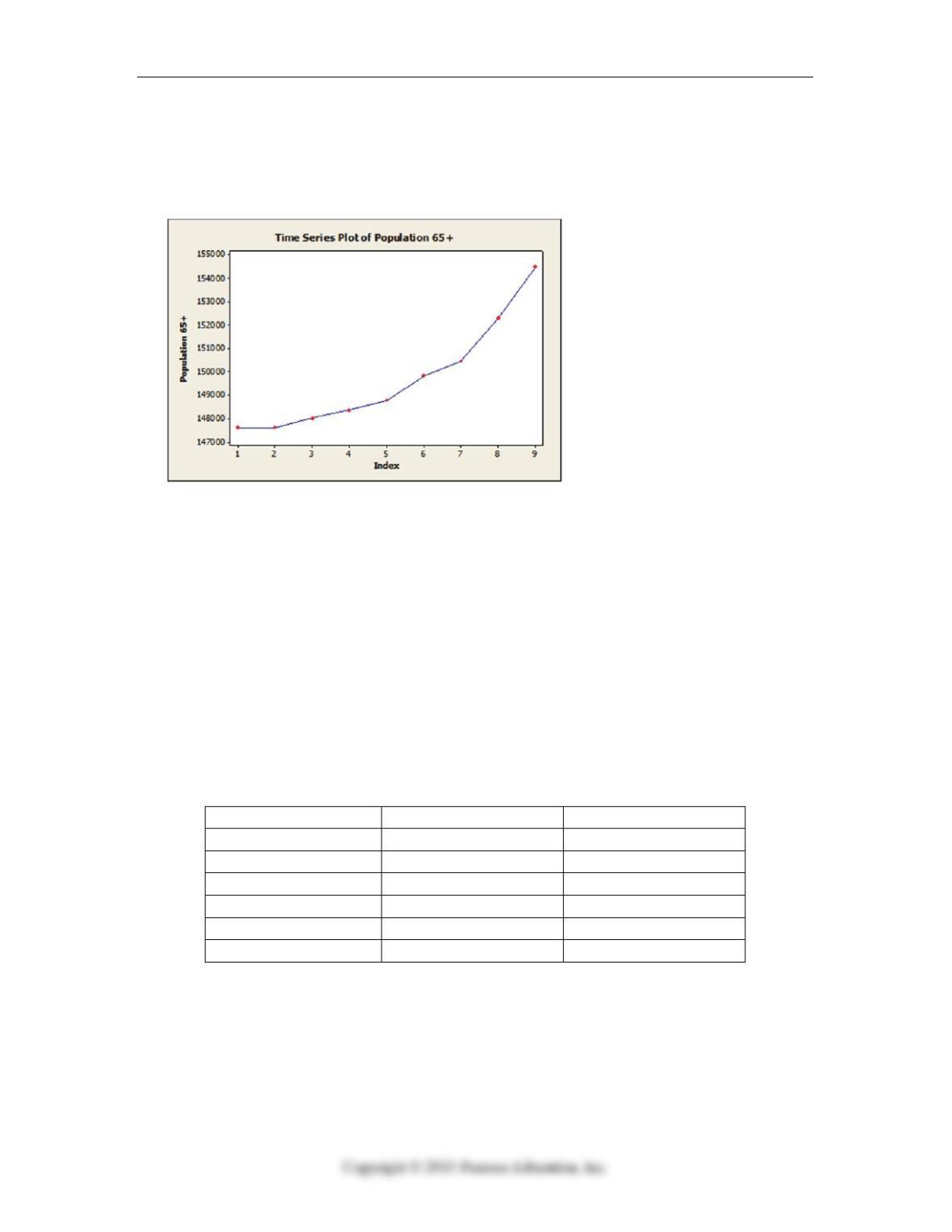
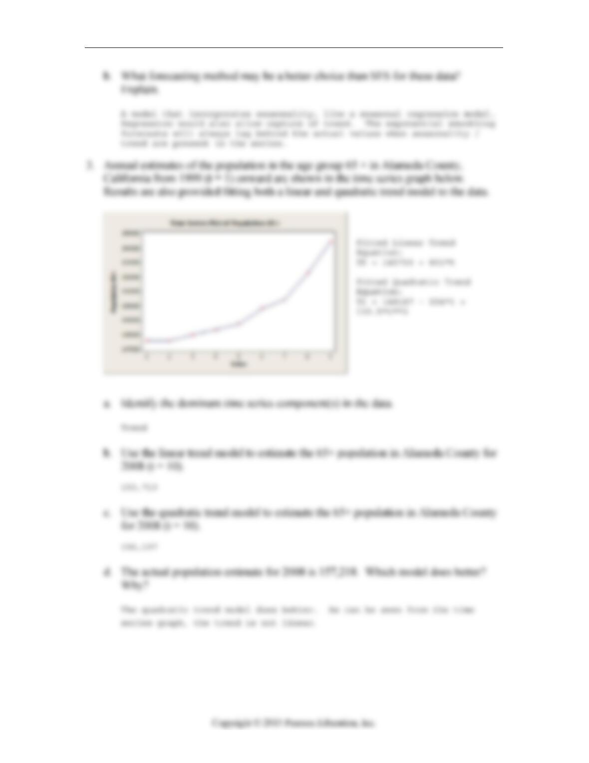
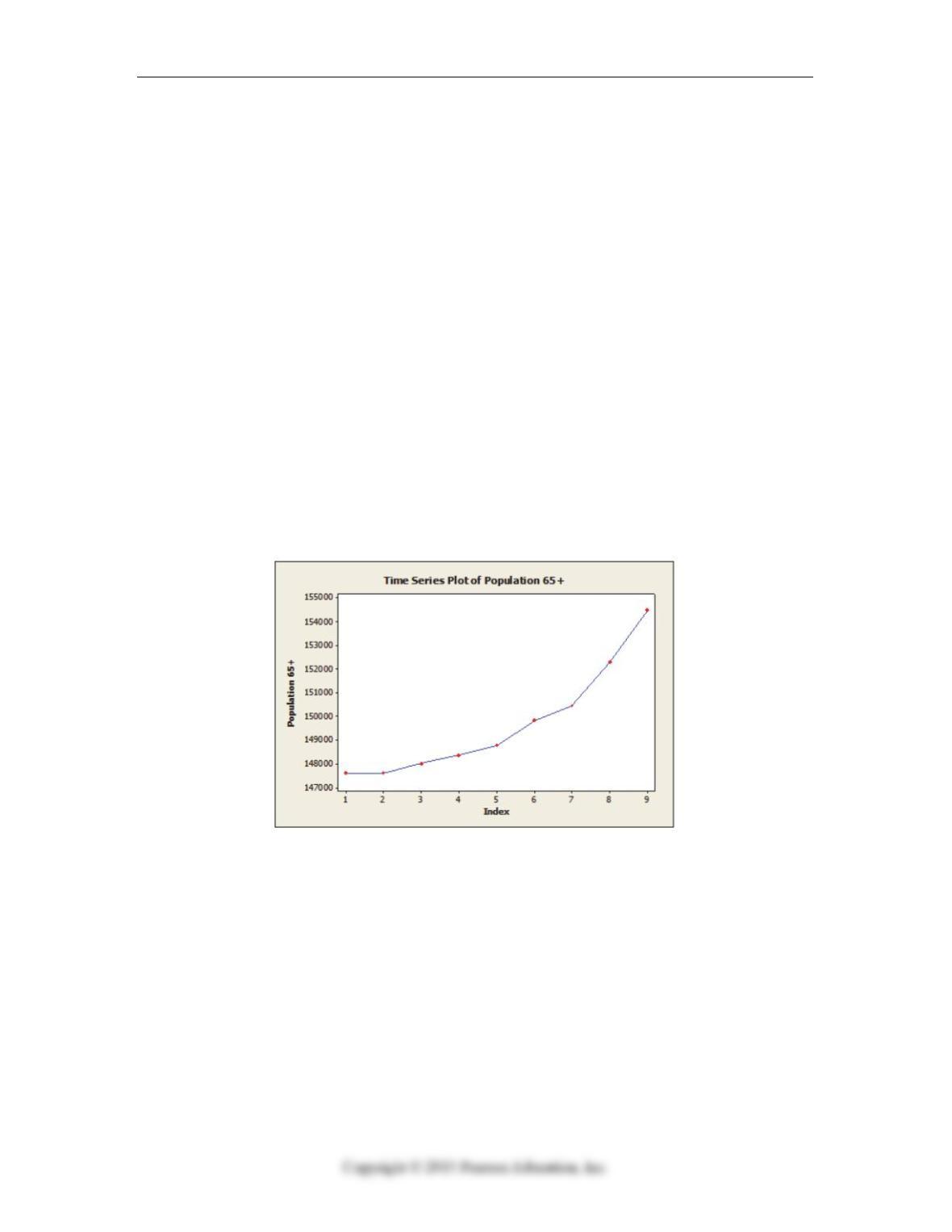
3. Annual estimates of the population in the age group 65 + in Alameda County,
California from 1999 (t = 1) onward are shown in the time series graph below.
Results are also provided fitting both a linear and quadratic trend model to the data.
Fitted Linear Trend
Equation:
Yt = 145703 + 801*t
Fitted Quadratic Trend
Equation:
Yt = 148187 – 554*t +
135.5*t**2
a. Identify the dominant time series component(s) in the data.
b. Use the linear model to estimate the 65+ population in Alameda County for 2008
(t = 10).
c. Use the quadratic model to estimate the 65+ population in Alameda County for
2008 (t = 10).
d. The actual population estimate for 2008 is 157,218. Which model does better?
Why?
19.4.5 Summarize forecasting error.
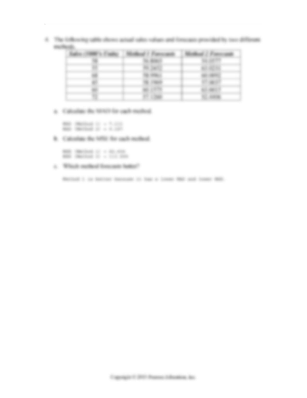
4. The following table shows actual sales values and forecasts provided by two different
methods.
Sales (1000’s Units) Method 1 Forecasts Method 2 Forecasts
58 56.8065 54.0577
55 59.2452 63.0231
68 58.9961 60.0092
45 58.1969 57.0037
60 60.1575 63.6015
72 57.1260 52.4406
a. Calculate the MAD for each method.
b. Calculate the MSE for each method.
c. Which method forecasts better?
Quiz A 19-3
19.5.6 Construct, interpret, and apply autoregressive models.
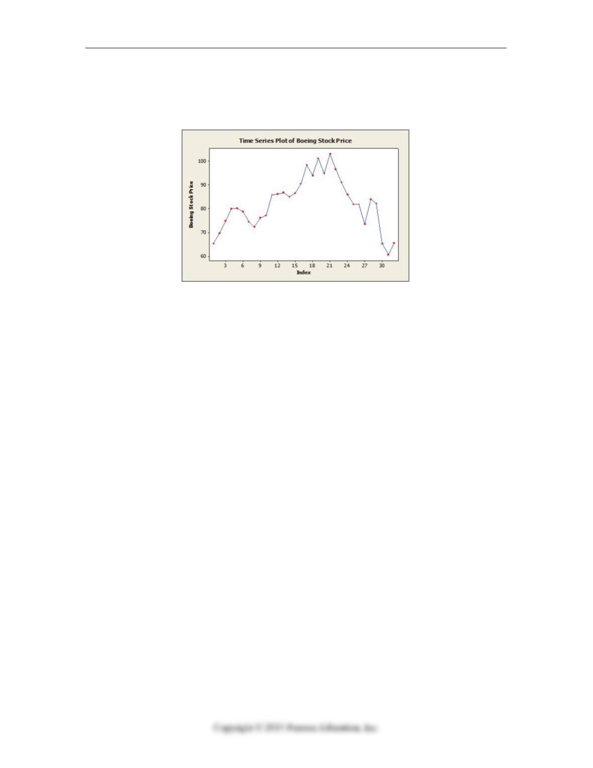
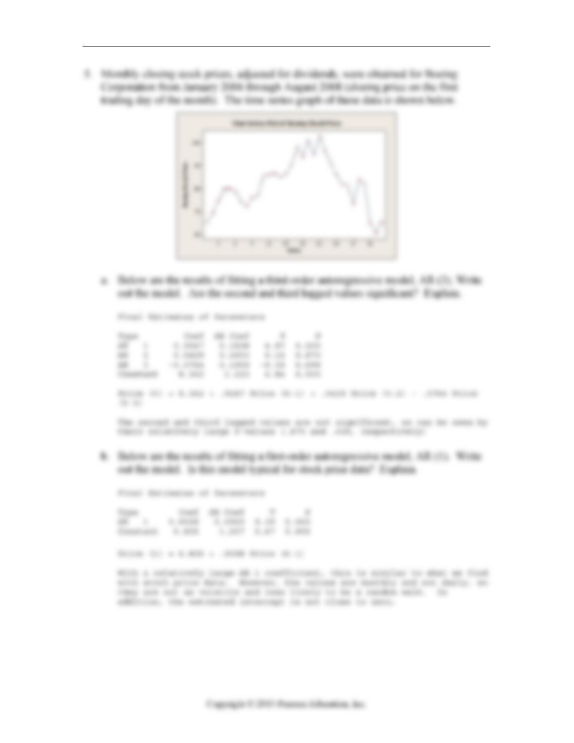
5. Monthly closing stock prices, adjusted for dividends, were obtained for Boeing
Corporation from January 2006 through August 2008 (closing price on the first
trading day of the month). The time series graph of these data is shown below.
a. Below are the results of fitting a third-order autoregressive model, AR (3). Write
out the model. Are the second and third lagged values significant? Explain.
Final Estimates of Parameters
Type Coef SE Coef T P
AR 1 0.9247 0.1898 4.87 0.000
AR 2 0.0429 0.2603 0.16 0.870
AR 3 -0.0764 0.1959 -0.39 0.699
Constant 8.362 1.223 6.84 0.000
b. Below are the results of fitting a first-order autoregressive model, AR (1). Write
out the model. Is this model typical for stock price data? Explain.
Final Estimates of Parameters
Type Coef SE Coef T P
AR 1 0.9098 0.0969 9.39 0.000
Constant 6.835 1.207 5.67 0.000
19-4 Chapter 19 Time Series Analysis
Chapter 19: Time Series Analysis – Quiz A – Key
Quiz A 19-5
19-6 Chapter 19 Time Series Analysis
Quiz A 19-7
19-8 Chapter 19 Time Series Analysis
Chapter 19: Time Series Analysis – Quiz B Name _____________________
19.7.8 Choose a forecasting method.
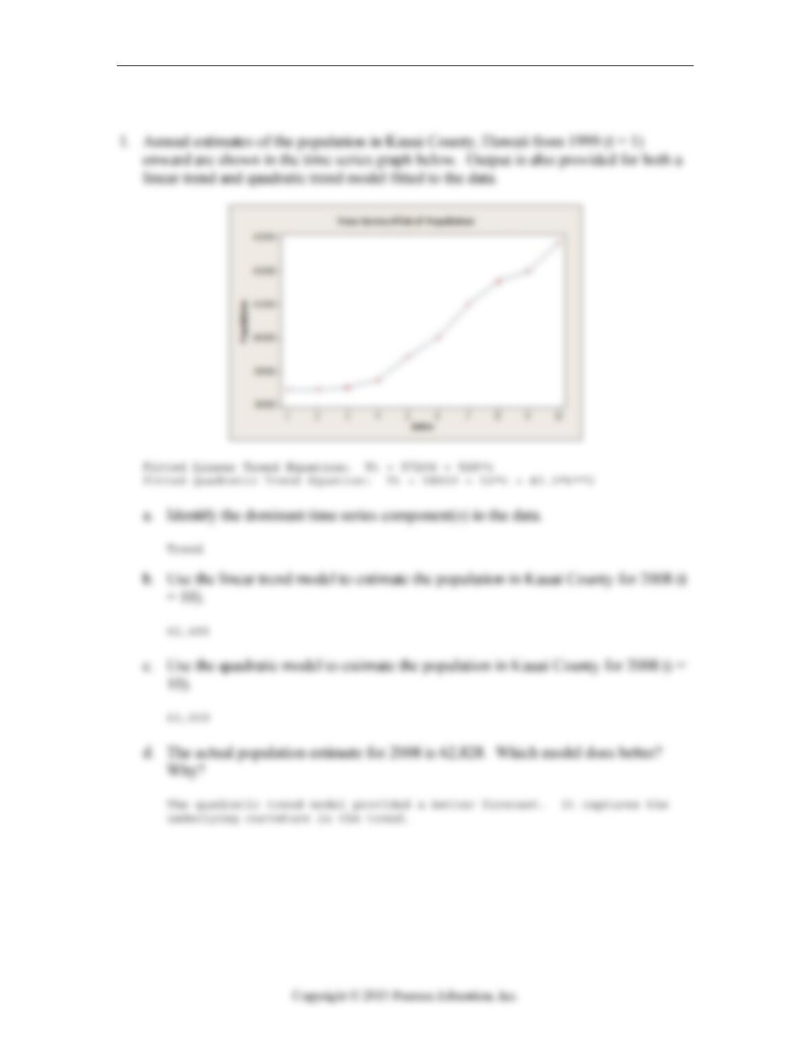
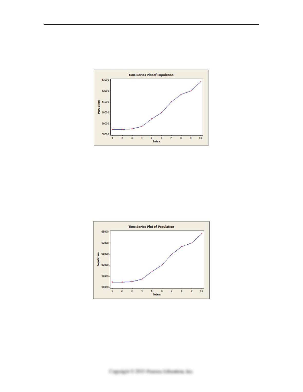
1. Annual estimates of the population in Kauai County, Hawaii from 1999 (t = 1)
onward are shown in the time series graph below. Output is also provided for both a
linear trend and quadratic trend model fitted to the data.
Fitted Linear Trend Equation: Yt = 57206 + 528*t
Fitted Quadratic Trend Equation: Yt = 58159 + 52*t + 43.3*t**2
a. Identify the dominant time series component(s) in the data.
b. Use the linear trend model to estimate the population in Kauai County for 2008 (t
= 10).
c. Use the quadratic model to estimate the population in Kauai County for 2008 (t =
10).
d. The actual population estimate for 2008 is 62,828. Which model does better?
Why?
Quiz B 19-9
19.2.3 Construct, interpret, and apply time series models.
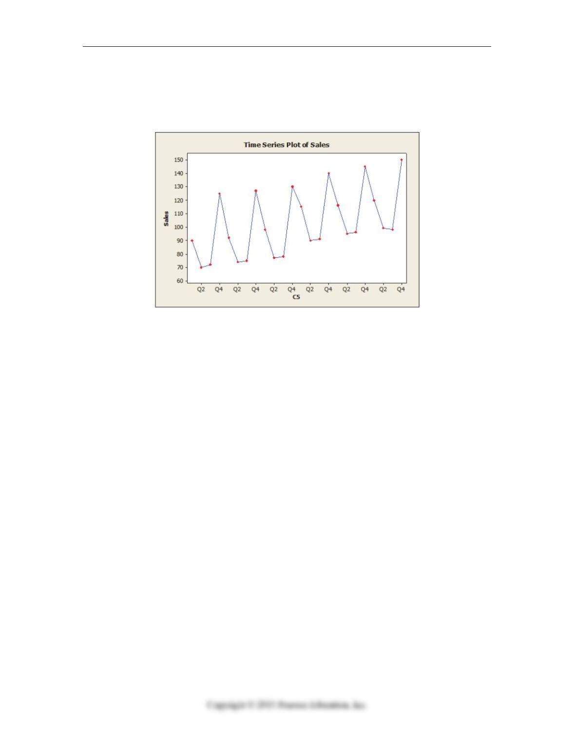
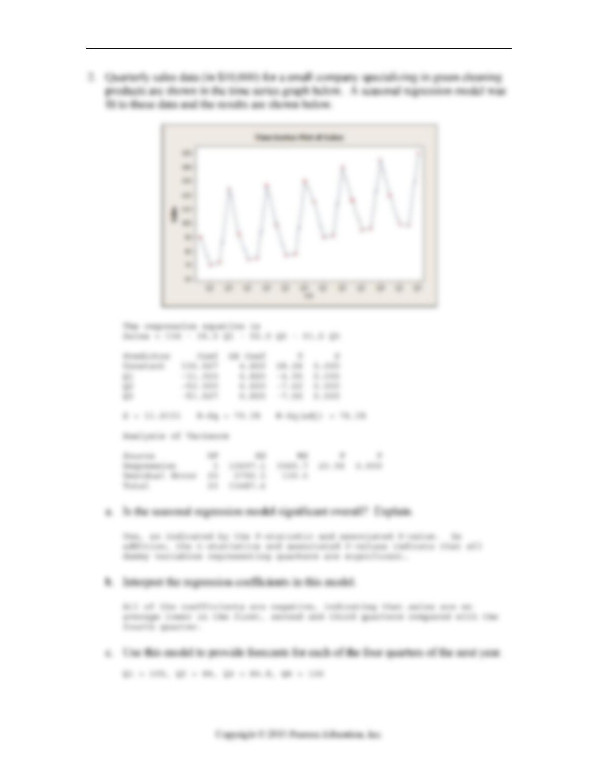
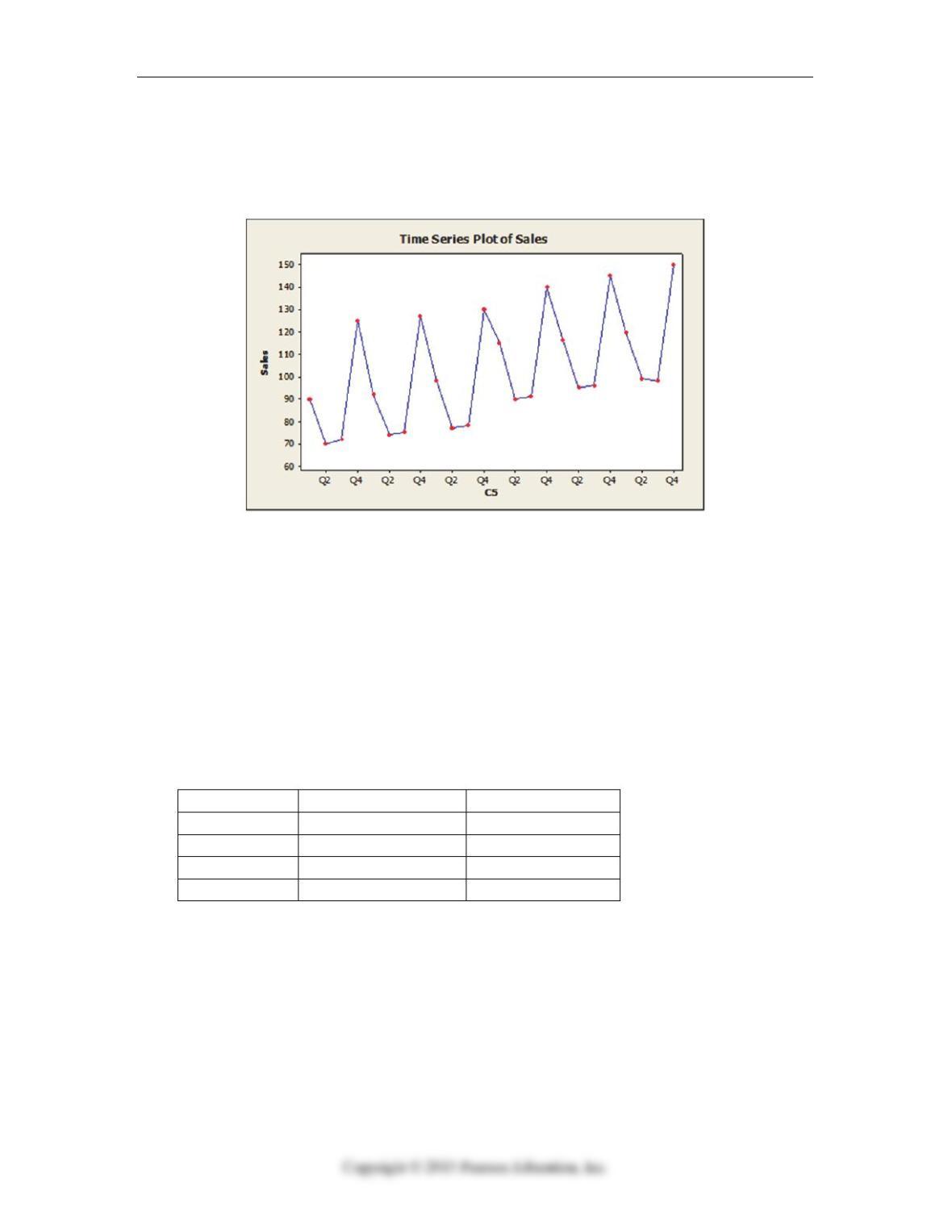
2. Quarterly sales data (in $10,000) for a small company specializing in green cleaning
products are shown in the time series graph below. A seasonal regression model was
fit to these data and the results are shown below.
The regression equation is
Sales = 136 – 31.0 Q1 – 52.0 Q2 – 51.2 Q3
Predictor Coef SE Coef T P
Constant 136.167 4.822 28.24 0.000
Q1 -31.000 6.820 -4.55 0.000
Q2 -52.000 6.820 -7.62 0.000
Q3 -51.167 6.820 -7.50 0.000
S = 11.8121 R-Sq = 79.3% R-Sq(adj) = 76.2%
Analysis of Variance
Source DF SS MS F P
Regression 3 10697.1 3565.7 25.56 0.000
Residual Error 20 2790.5 139.5
Total 23 13487.6
a. Is the seasonal regression model significant overall? Explain.
b. Interpret the regression coefficients in this model.
c. Use this model to provide forecasts for each of the four quarters of the next year.
19-10 Chapter 19 Time Series Analysis
19.2.2 Identify components of time series.
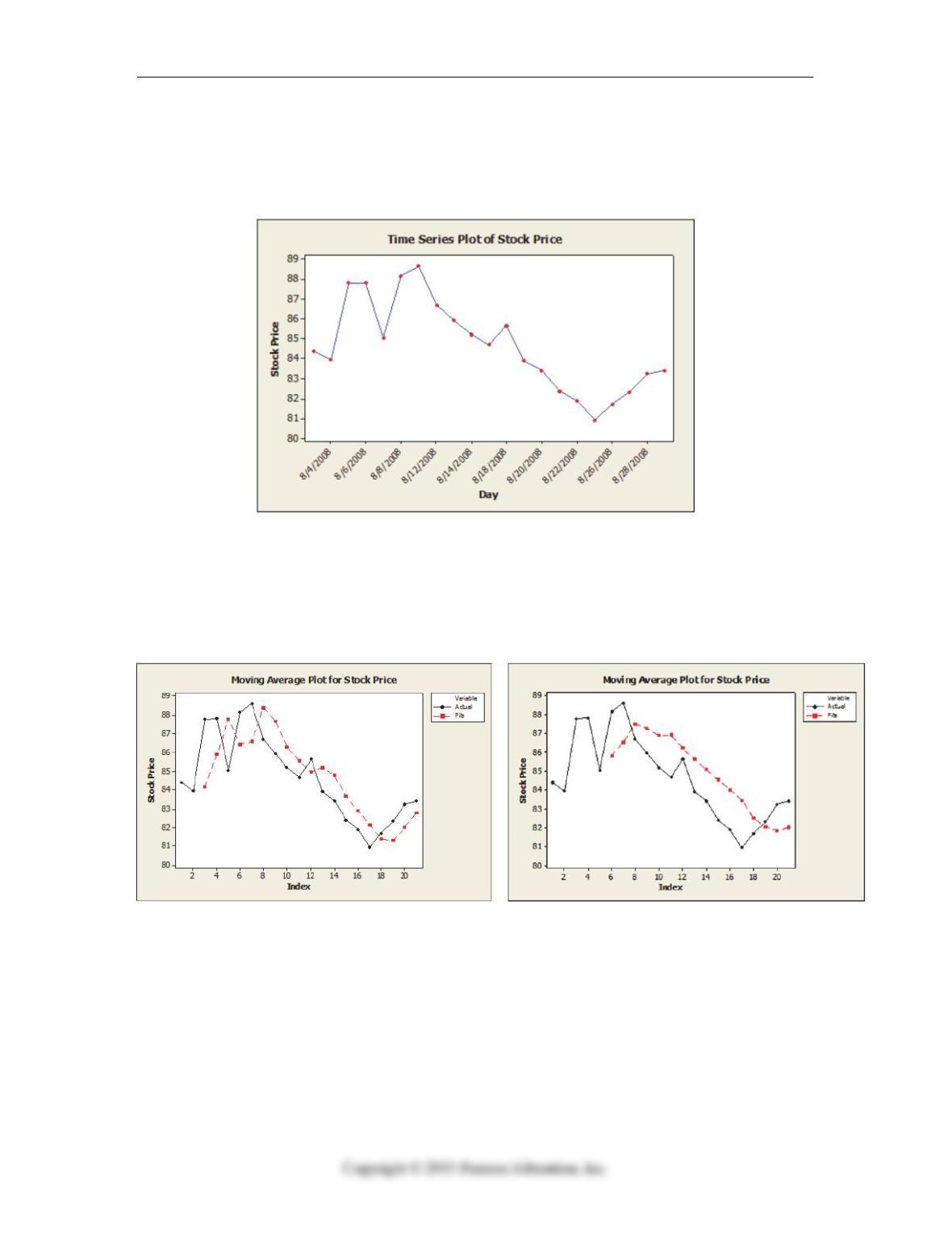
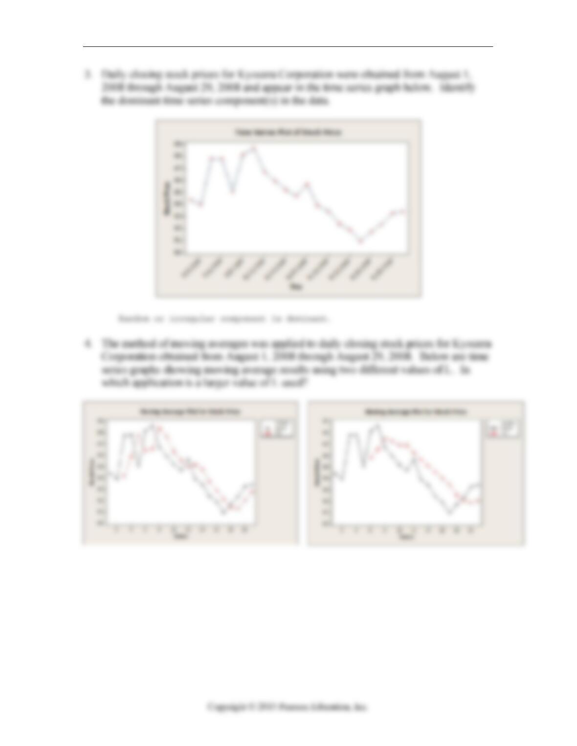
3. Daily closing stock prices for Kyocera Corporation were obtained from August 1,
2008 through August 29, 2008 and appear in the time series graph below. Identify
the dominant time series component(s) in the data.
19.3.3 Construct, interpret, and apply time series models.
4. The method of moving averages was applied to daily closing stock prices for Kyocera
Corporation obtained from August 1, 2008 through August 29, 2008. Below are time
series graphs showing moving average results using two different values of L. In
which application is a larger value of L used?
Quiz B 19-11
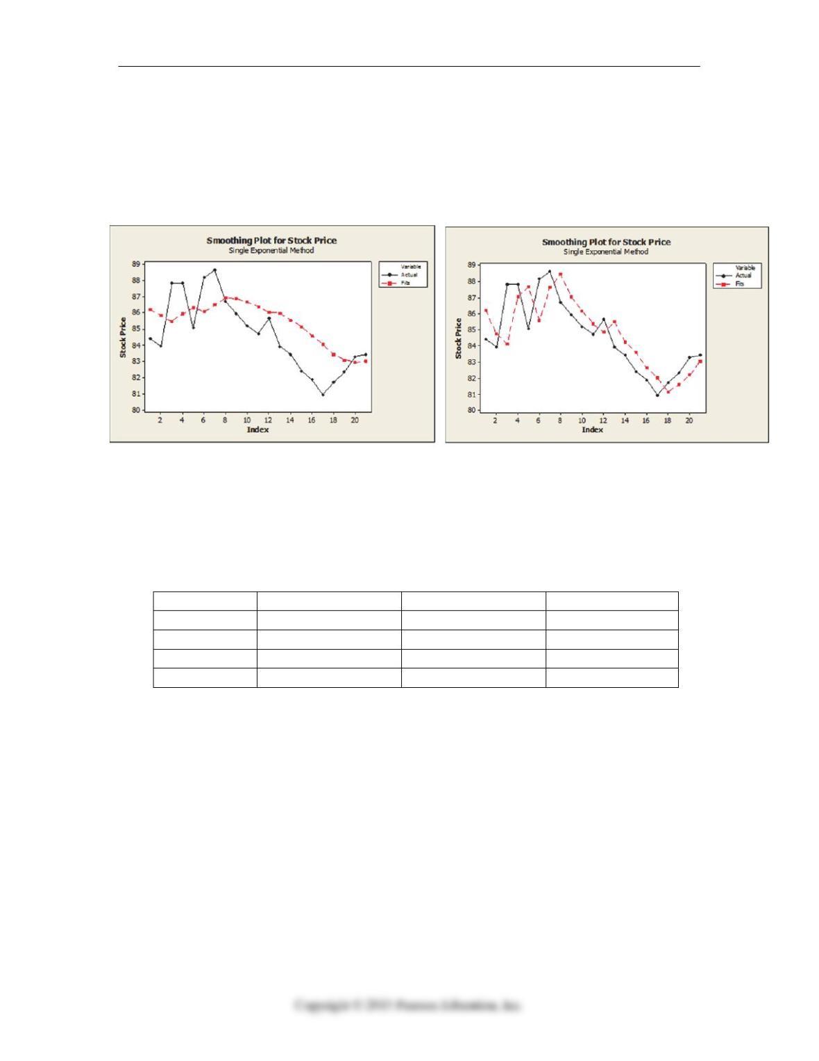
19.3.4 Smooth time series models.
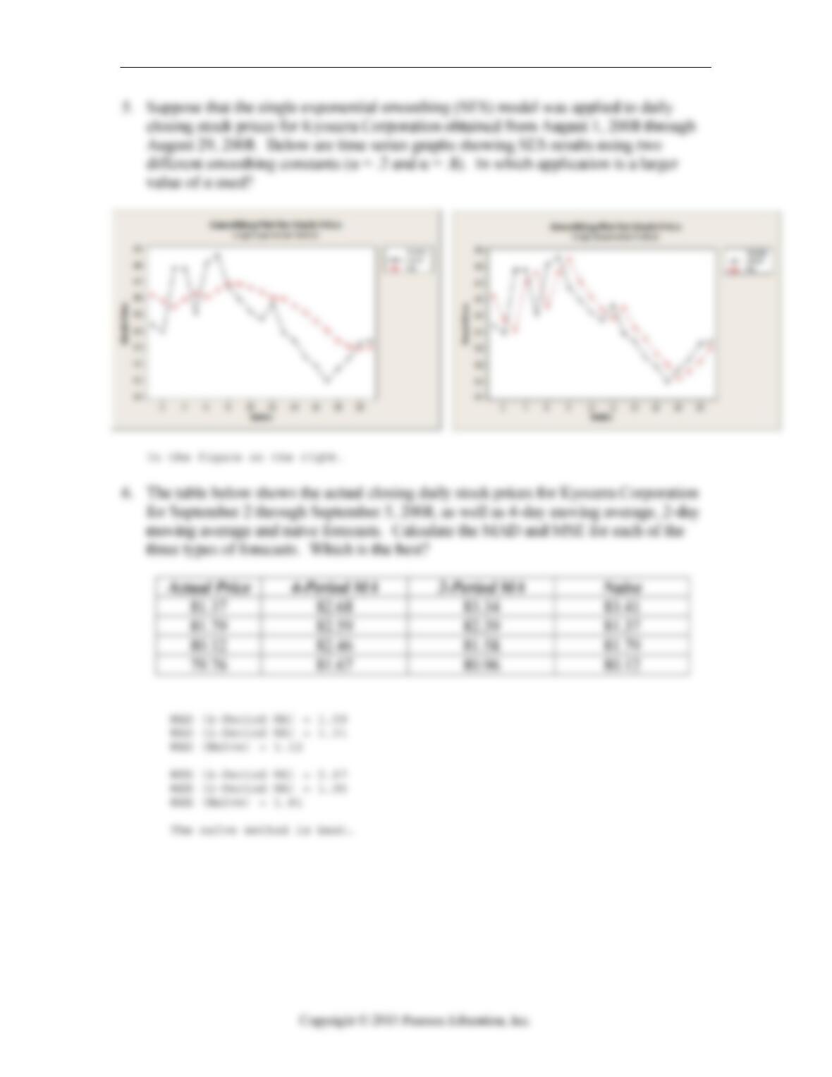
5. Suppose that the single exponential smoothing (SES) model was applied to daily
closing stock prices for Kyocera Corporation obtained from August 1, 2008 through
August 29, 2008. Below are time series graphs showing SES results using two
different smoothing constants (α = .2 and α = .8). In which application is a larger
value of α used?
19.4.5 Summarize forecasting error.
6. The table below shows the actual closing daily stock prices for Kyocera Corporation
for September 2 through September 5, 2008, as well as 4-day moving average, 2-day
moving average and naïve forecasts. Calculate the MAD and MSE for each of the
three types of forecasts. Which is the best?
Actual Price 4-Period MA 2-Period MA Naive
81.37 82.68 83.34 83.41
81.79 82.59 82.39 81.37
80.12 82.46 81.58 81.79
79.76 81.67 80.96 80.12
19-12 Chapter 19 Time Series Analysis
Chapter 19: Time Series Analysis – Quiz B – Key
Quiz B 19-13
19-14 Chapter 19 Time Series Analysis
Quiz B 19-15
19-16 Chapter 19 Time Series Analysis
Chapter 19: Time Series Analysis Name________________________
Quiz C – Multiple Choice
19.2.2 Identify components of a time series.
1. American Spinners, a large automobile parts supplier, keeps track of the demand for a
particular part needed by its customers, automobile manufacturers. The time series
plot below shows monthly demand for this part (in thousands) for a five year period.
The dominant component in this time series is
A. cyclicity.
B. randomness.
C. seasonality.
D. systematic.
E. None of the above.
Quiz C 19-17
19.2.2 Identify components of a time series.
2. Annual estimates of the population in Kauai County, Hawaii from 1999 (t = 1)
onward are shown in the time series graph below. The dominant component in this
time series is
A. cyclicity.
B. randomness.
C. seasonality.
D. trend.
E. None of the above.
19.7.8. Choose a forecasting method.
3. Annual estimates of the population in Kauai County, Hawaii from 1999 (t = 1)
onward are shown in the graph below. The most appropriate forecasting method for
this series is
A. single exponential smoothing.
B. quadratic trend.
C. moving average.
D. naïve.
E. linear trend.

19-18 Chapter 19 Time Series Analysis
19.4.5 Summarize forecast error.
4. The following table shows actual sales values and forecasts. The MAD for the
forecasting method used is
Sales (1000’s Units) Forecasts
58 56.8065
55 59.2452
68 58.9961
45 58.1969
60 60.1575
72 57.1260
A. 7.111
B. 9.187
C. 82.656
D. 113.899
E. None of the above.
19.4.5 Summarize forecast error.
5. The following table shows actual sales values and forecasts. The MSE for the
forecasting method used is
Sales (1000’s Units) Forecasts
58 56.8065
55 59.2452
68 58.9961
45 58.1969
60 60.1575
72 57.1260
A. 7.111
B. 9.187
C. 82.656
D. 113.899
E. None of the above.

Quiz C 19-19
19.6.7 Construct, interpret, and apply multiple regression-based models.
6. A seasonal regression model was fit to quarterly sales data (in $10,000) for a small
company specializing in green cleaning products. The results are shown below.
Which of the following statements is true?
The regression equation is
Sales = 136 – 31.0 Q1 – 52.0 Q2 – 51.2 Q3
Predictor Coef SE Coef T P
Constant 136.167 4.822 28.24 0.000
Q1 -31.000 6.820 -4.55 0.000
Q2 -52.000 6.820 -7.62 0.000
Q3 -51.167 6.820 -7.50 0.000
S = 11.8121 R-Sq = 79.3% R-Sq(adj) = 76.2%
Analysis of Variance
Source DF SS MS F P
Regression 3 10697.1 3565.7 25.56 0.000
Residual Error 20 2790.5 139.5
Total 23 13487.6
A. The seasonal regression model is significant in explaining sales as indicated by
the F-statistic and associated P-value.
B. The seasonal regression model explains 79.3% of the variation in sales.
C. The t-statistics and associated P-values indicate that all dummy variables
representing quarters are significant.
D. Both A and B.
E. All of the above.

19-20 Chapter 19 Time Series Analysis
19.6.7 Construct, interpret, and apply multiple regression-based models.
7. A seasonal regression model was fit to quarterly sales data (in $10,000) for a small
company specializing in green cleaning products. The results are shown below. The
regression coefficients in the seasonal regression model indicate that sales are on
average
The regression equation is
Sales = 136 – 31.0 Q1 – 52.0 Q2 – 51.2 Q3
Predictor Coef SE Coef T P
Constant 136.167 4.822 28.24 0.000
Q1 -31.000 6.820 -4.55 0.000
Q2 -52.000 6.820 -7.62 0.000
Q3 -51.167 6.820 -7.50 0.000
S = 11.8121 R-Sq = 79.3% R-Sq(adj) = 76.2%
A. lower in the first, second and third quarters compared with the fourth quarter.
B. lowest in the fourth quarter.
C. higher in the first, second and third quarters compared with the fourth quarter.
D. lowest in the first quarter.
E. None of the above.
19.6.7 Construct, interpret, and apply multiple regression-based models.
8. Annual estimates of the population in the age group 65 + in Alameda County,
California from 1999 (t = 1) onward are used to estimate the following quadratic
trend model: Yt = 148187 – 554*t + 135.5*t**2. Using this model, the estimate
for 2008 is
A. 157,218.
B. 156,197.
C. 153,713.
D. 161,312.
E. None of the above.

Quiz C 19-21
19.5.6 Construct, interpret, and apply autoregressive models.
9. A third-order autoregressive model, AR (3) was fit to monthly closing stock prices,
adjusted for dividends, of Boeing Corporation from January 2006 through August
2008 (closing price on the first trading day of the month). Based on the results
shown below, the estimated model is
Final Estimates of Parameters
Type Coef SE Coef T P
AR 1 0.9247 0.1898 4.87 0.000
AR 2 0.0429 0.2603 0.16 0.870
AR 3 -0.0764 0.1959 -0.39 0.699
Constant 8.362 1.223 6.84 0.000
A. Price (t) = 1.223 + .1898 Price (t-1) + .2603 Price (t-2) + 1959 Price (t-3)
B. Price (t) = 8.362 – .0764 Price (t-1) + .0429 Price (t-2) + .9247 Price (t-3)
C. Price (t) = 1.223 + .1959 Price (t-1) + .2603 Price (t-2) + .1898 Price (t-3)
D. Price (t) = 8.362 + .9247 Price (t-1) + .0429 Price (t-2) – .0764 Price (t-3)
E. None of the above.
19.5.6 Construct, interpret, and apply autoregressive models.
10. A third-order autoregressive model, AR (3) was fit to monthly closing stock prices,
adjusted for dividends, of Boeing Corporation from January 2006 through August
2008 (closing price on the first trading day of the month). Based on the results
shown below, at α = .05 which of the following statement is true?
Final Estimates of Parameters
Type Coef SE Coef T P
AR 1 0.9247 0.1898 4.87 0.000
AR 2 0.0429 0.2603 0.16 0.870
AR 3 -0.0764 0.1959 -0.39 0.699
Constant 8.362 1.223 6.84 0.000
A. the first lagged variable is significant.
B. the second lagged variable is significant.
C. the first lagged variable is significant.
D. Both B and C.
E. All of the above.

19-22 Chapter 19 Time Series Analysis
Chapter 19: Time Series Analysis – Quiz C – Key

Quiz D 19-23
Chapter 19: Time Series Analysis Name________________________
Quiz D – Multiple Choice
19.3.4 Smooth time series models.
1. The table below shows the actual closing daily stock prices for Kyocera Corporation
for September 2 through September 4, 2008. What is the 2-day moving average
forecast for September 5?
Date Actual Price 2-Period MA Forecast
Sept. 2 81.37 83.34
Sept. 3 81.79 82.39
Sept. 4 80.12 81.58
Sept. 5
A. 80.96
B. 79.94
C. 82.87
D. 80.12
E. 81.99
19.3.4 Smooth time series models.
2. The table below shows the actual closing daily stock prices for Kyocera Corporation
for September 2 through September 5, 2008. Suppose the forecast for Sept. 2 is
81.88. Using SES (single exponential smoothing) with a smoothing constant of 0.2 (α
= 0.2), what is the forecast for Sept. 3?
Date Actual Price
Sept. 2 81.37
Sept. 3 81.79
Sept. 4 80.12
Sept. 5 79.76
A. 81.86
B. 81.78
C. 81.81
D. 81.55
E. None of the above.
19-24 Chapter 19 Time Series Analysis
19.7.8 Choose a forecasting method.
3. Quarterly sales data (in $10,000) for a small company specializing in green cleaning
products are shown in the time series graph below. The forecasting method that
would likely fit these data the best is
A. single exponential smoothing.
B. linear trend.
C. seasonal regression model.
D. moving average.
E. naive.
19.4.5 Summarize forecasting error.
4. The table below shows the actual closing daily stock prices for Kyocera Corporation
for September 2 through September 5, 2008, as well as 4-day moving average and
naïve forecasts. The MAD for the Naïve method is 1.22. What is the MAD for the 4-
period MA and how does it compare with the Naïve?
Actual Price 4-Period MA Naive
81.37 82.68 83.41
81.79 82.59 81.37
80.12 82.46 81.79
79.76 81.67 80.12
A. MAD (4-Period MA) is 1.59; the Naïve method is better.
B. MAD (4-Period MA) is 1.59; the Naïve method is worse.
C. MAD (4-Period MA) is 1.81; the Naïve method is better.
D. MAD (4-Period MA) is 1.01; the Naïve method is worse.
E. MAD (4-Period MA) is 2.87; the Naïve method is worse.

Quiz D 19-25
19.7.3 Construct, interpret, and apply time series models.
5. A seasonal regression model was fit to quarterly sales data (in $10,000) for a small
company specializing in green cleaning products. The results are shown below.
What is the forecast (in $10,000) for the second quarter of the next year?
The regression equation is
Sales = 136 – 31.0 Q1 – 52.0 Q2 – 51.2 Q3
Predictor Coef SE Coef T P
Constant 136.167 4.822 28.24 0.000
Q1 -31.000 6.820 -4.55 0.000
Q2 -52.000 6.820 -7.62 0.000
Q3 -51.167 6.820 -7.50 0.000
S = 11.8121 R-Sq = 79.3% R-Sq(adj) = 76.2%
A. 105
B. 84
C. 52
D. 136
E. 31
19.7.3 Construct, interpret, and apply time series models.
6. A quadratic trend model was fit to data on annual estimates of the population in the
age group 65 + in Alameda County, California from 1999 (t = 1) onward. The results
are shown below. Using this model, the estimate of population in the 65+ age group
in Alameda County for 2008 (t = 10) is
Fitted Trend Equation: Yt = 148187 – 554*t + 135.5*t**2
A. 153,713
B. 148,187
C. 161,737
D. 156,197
E. 167,277
19-26 Chapter 19 Time Series Analysis
19.5.6 Construct, interpret, and apply autoregressive models.
7. A first-order autoregressive model, AR (3) was fit to monthly closing stock prices,
adjusted for dividends, of Boeing Corporation from January 2006 through August
2008 (closing price on the first trading day of the month). Based on the results
shown below, the estimated model is
Final Estimates of Parameters
Type Coef SE Coef T P
AR 1 0.9098 0.0969 9.39 0.000
Constant 6.835 1.207 5.67 0.000
A. Price (t) = 6.835 + .9098 Price (t-1)
B. Price (t) = 0.0969 + 1.207 Price (t-1)
C. Price (t) = 1.207 + 0.0969 Price (t-1)
D. Price (t) = 6.835 + 1.207 Price (t-1)
E. Price (t) = 6.835 – 0.9098 Price (t-1)
19.2.2 Identify components of time series.
8. Annual estimates of the population in the age group 65 + in Alameda County,
California from 1999 (t = 1) onward are shown in the time series graph below. The
dominant component in the time series is
A. cyclicity
B. randomness.
C. seasonality.
D. trend.
E. None of the above.
Quiz D 19-27
19.2.2 Identify components of time series.
9. Daily closing stock prices for Kyocera Corporation were obtained from August 1,
2008 through August 29, 2008 and appear in the time series graph below. The
dominant component in this time series is
A. trend.
B. irregular.
C. seasonality.
D. systematic.
E. None of the above.
19-28 Chapter 19 Time Series Analysis
19.3.3 Construct, interpret, and apply time series models.
10. Suppose that the single exponential smoothing (SES) model was applied to data
measuring demand for a particular part needed by customer with results as shown
below. The likely value used for α is
A. 1.0
B. 0.9
C. 0.8
D. 0.5
E. 0.2

Quiz D 19-29
Chapter 19: Time Series Analysis – Quiz D – Key