Time-Series Forecasting 16-1
CHAPTER 16: TIME-SERIES FORECASTING
1. The effect of an unpredictable, rare event will be contained in the ___________ component.
a) trend
b) cyclical
c) irregular
d) seasonal
2. The overall upward or downward pattern of the data in an annual time series will be
contained in the ____________ component.
a) trend
b) cyclical
c) irregular
d) seasonal
3. The fairly regular fluctuations that occur within each year would be contained in the
_________________ component.
a) trend
b) cyclical
c) irregular
d) seasonal
4. The annual multiplicative time-series model does not possess _______ component.
a) a trend
b) a cyclical
c) an irregular
d) a seasonal
ANSWER:
16-2 Time-Series Forecasting
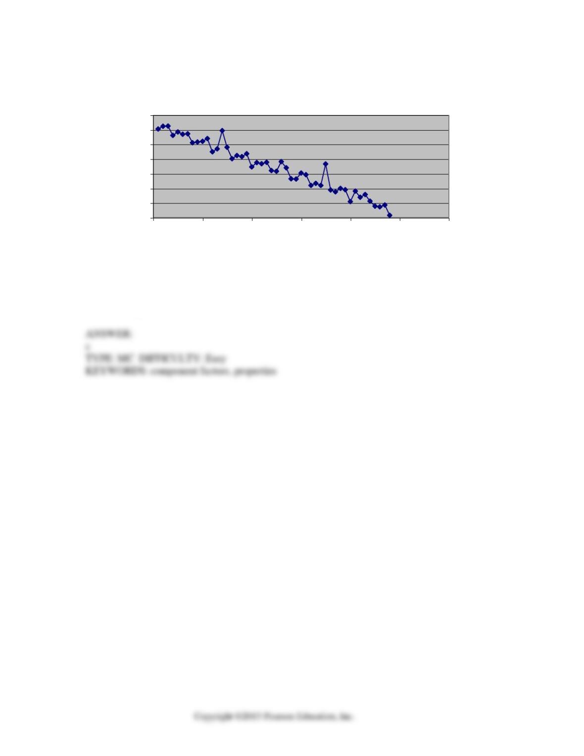
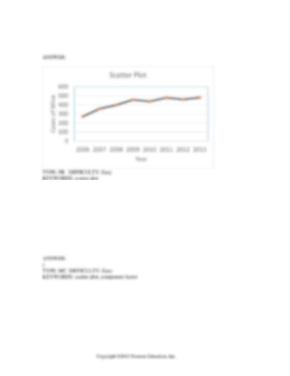
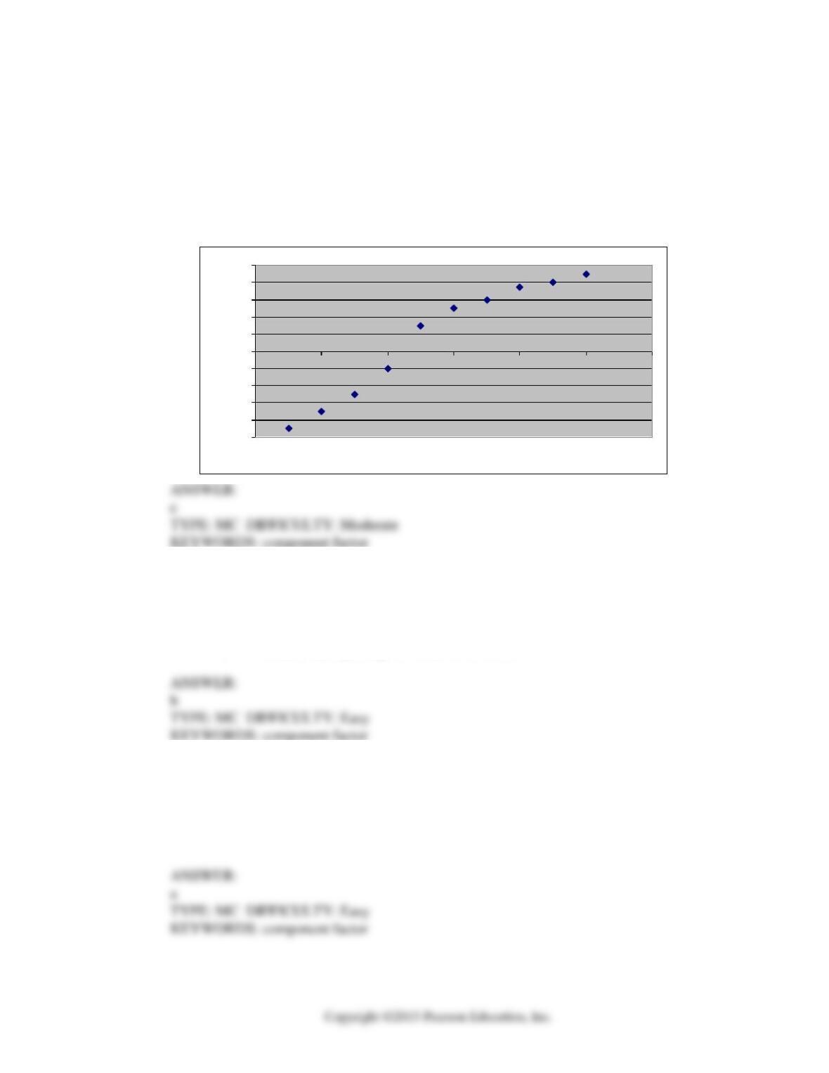
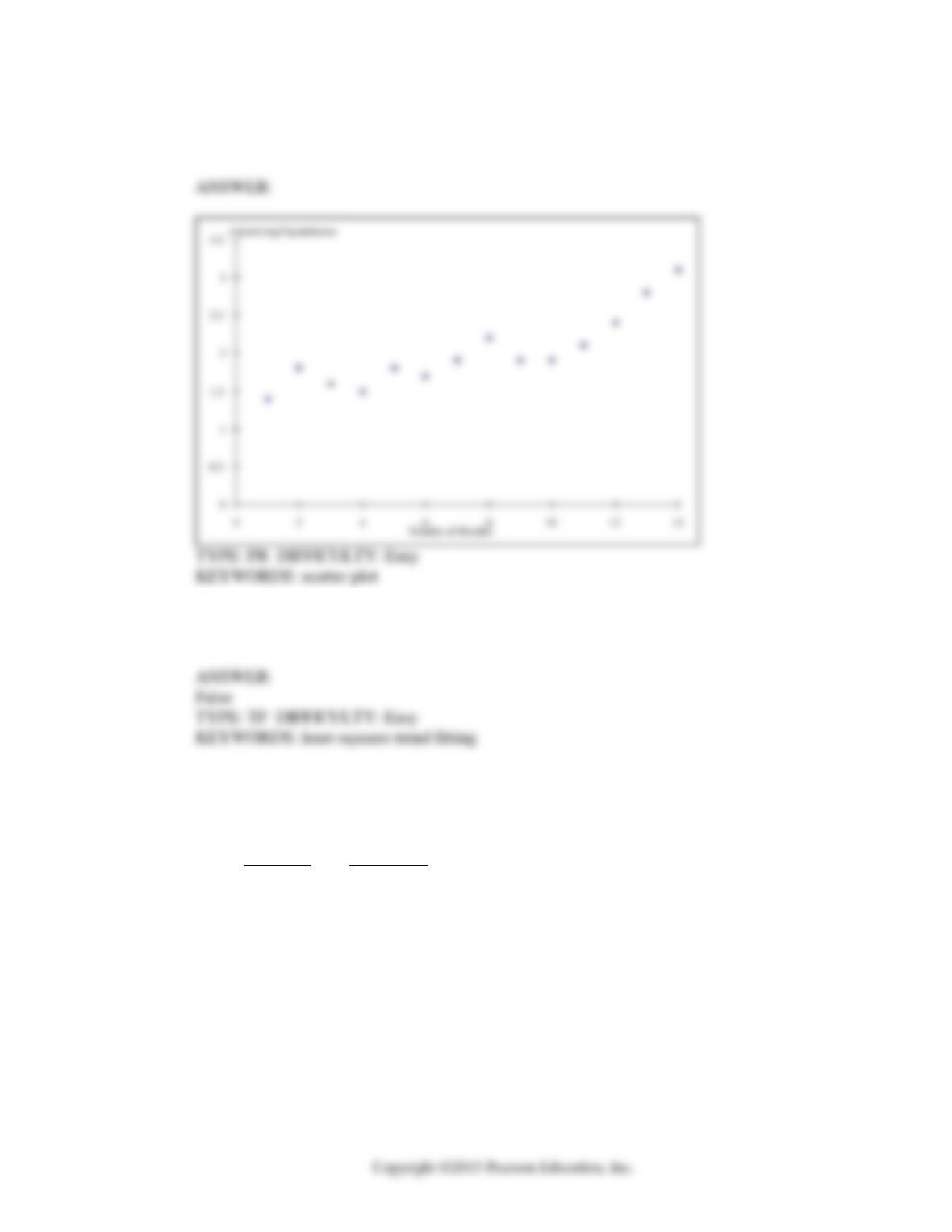
5. Based on the following scatter plot, which of the time-series components is not present in
this quarterly time series?
0
50
100
150
200
250
300
350
010 20 30 40 50 60
Quarters
Stoc k Returns
a. Trend
b. Seasonal
c. Cyclical
d. Irregular
Time-Series Forecasting 16-3
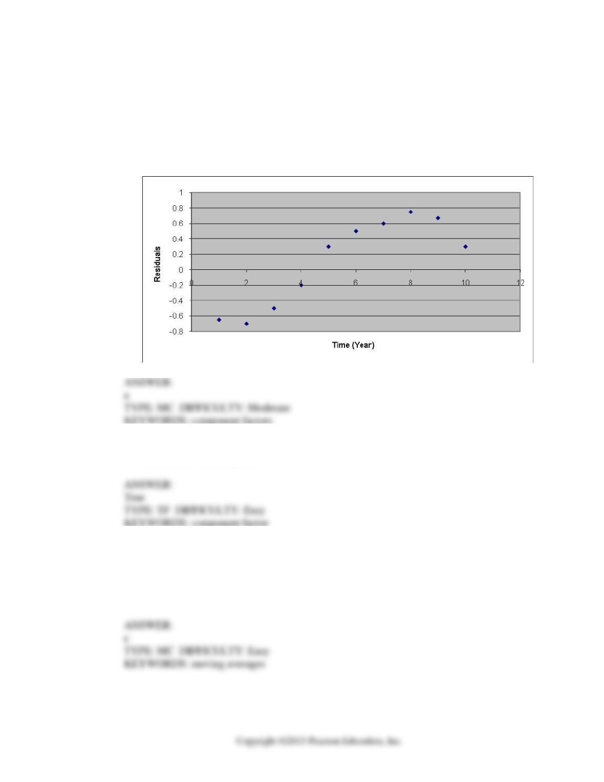
6. After estimating a trend model for annual time-series data, you obtain the following residual
plot against time, the problem with your model is that:
a) The cyclical component has not been accounted for.
b) The seasonal component has not been accounted for.
c) The trend component has not been accounted for.
d) The irregular component has not been accounted for.
7. True or False: A trend is a persistent pattern in annual time-series data that has to be
followed for several years.
8. The method of moving averages is used
a) to plot a series.
b) to exponentiate a series.
c) to smooth a series.
d) in regression analysis.
16-4 Time-Series Forecasting
9. Which of the following methods should not be used for short-term forecasts into the future?
a) Exponential smoothing
b) Moving averages
c) Linear trend model
d) Autoregressive modeling
10. Which of the following statements about moving averages is not true?
a) It can be used to smooth a series.
b) It gives equal weight to all values in the computation.
c) It is simpler than the method of exponential smoothing.
d) It gives greater weight to more recent data.
11. True or False: Given a data set with 15 yearly observations, a 3-year moving average will
have fewer observations than a 5-year moving average.
12. True or False: Given a data set with 15 yearly observations, there are only thirteen 3-year
moving averages.
13. True or False: Given a data set with 15 yearly observations, there are only seven 9-year
moving averages.
Time-Series Forecasting 16-5
14. Which of the following is not an advantage of exponential smoothing?
a) It enables you to perform one-period ahead forecasting.
b) It enables you to perform more than one-period ahead forecasting.
c) It enables you to smooth out seasonal components.
d) It enables you to smooth out cyclical components.
15. When using the exponentially weighted moving average for purposes of forecasting rather
than smoothing,
a) the previous smoothed value becomes the forecast.
b) the current smoothed value becomes the forecast.
c) the next smoothed value becomes the forecast.
d) None of the above.
16. Which of the following statements about the method of exponential smoothing is not true?
a) It gives greater weight to more recent data.
b) It can be used for forecasting.
c) It uses all earlier observations in each smoothing calculation.
d) It gives greater weight to the earlier observations in the series.
17. True or False: If a time series does not exhibit a long-term trend, the method of exponential
smoothing may be used to obtain short-term predictions about the future.
16-6 Time-Series Forecasting
18. A model that can be used to make predictions about long-term future values of a time series
is a) linear trend.
b) quadratic trend.
c) exponential trend.
d) All of the above.
19. You need to decide whether you should invest in a particular stock. You would like to invest
if the price is likely to rise in the long run. You have data on the daily mean price of this
stock over the past 12 months. Your best action is to
a) compute moving averages
b) perform exponential smoothing
c) estimate a least square trend model
d) compute the MAD statistic
20. When a time series appears to be increasing at an increasing rate, such that percentage
difference from value to value is constant, the appropriate model to fit is the
a. linear trend.
b. quadratic trend.
c. exponential trend.
d. None of the above.
21. The method of least squares is used on time-series data for
a) eliminating irregular movements.
b) deseasonalizing the data.
c) obtaining the trend equation.
d) exponentially smoothing a series.
Time-Series Forecasting 16-7
22. True or False: A least squares linear trend line is just a simple regression line with the years
recoded.
23. True or False: The method of least squares may be used to estimate both linear and
curvilinear trends.
24. Microsoft Excel was used to obtain the following quadratic trend equation:
Sales = 100 – 10X + 15X2.
The data used was from 2004 through 2013 coded 0 to 9. The forecast for 2014 is
__________.
25. The manager of a company believed that her company’s profits were following an
exponential trend. She used Microsoft Excel to obtain a prediction equation for the logarithm
(base 10) of profits:
log10(Profits) = 2 + 0.3X
The data she used were from 2007 through 2012 coded 0 to 5. The forecast for 2013 profits
is __________.
26. A first-order autoregressive model for stock sales is:
Salesi = 800 + 1.2(Sales)i-1.
If sales in 2012 is 6,000, the forecast of sales for 2013 is __________.
16-8 Time-Series Forecasting
27. A second-order autoregressive model for average mortgage rate is:
Ratei = – 2.0 + 1.8(Rate)i-1 – 0.5 (Rate)i-2.
If the average mortgage rate in 2012 was 7.0, and in 2011 was 6.4, the forecast for 2013 is
__________.
28. A second-order autoregressive model for average mortgage rate is:
Ratei = – 2.0 + 1.8(Rate)i-1 – 0.5 (Rate)i-2.
If the average mortgage rate in 2012 was 7.0, and in 2011 was 6.4, the forecast for 2014 is
__________.
29. In selecting an appropriate forecasting model, the following approaches are suggested:
a) Perform a residual analysis.
b) Measure the size of the forecasting error.
c) Use the principle of parsimony.
d) All of the above.
30. To assess the adequacy of a forecasting model, one measure that is often used is
a) quadratic trend analysis.
b) the MAD.
c) exponential smoothing.
d) moving averages.
31. True or False: MAD is the summation of the residuals divided by the sample size.
ANSWER:
Time-Series Forecasting 16-9
32. True or False: The principle of parsimony indicates that the simplest model that gets the job
done adequately should be used.
33. True or False: In selecting a forecasting model, you should perform a residual analysis.
34. True or False: Each forecast using the method of exponential smoothing depends on all the
previous observations in the time series.
35. True or False: The MAD is a measure of the mean of the absolute discrepancies between the
actual and the fitted values in a given time series.
SCENARIO 16-1
The number of cases of chardonnay wine sold by a Paso Robles winery in an 8-year period
follows.
Year Cases of Wine
2006 270
2007 356
2008 398
2009 456
2010 438
2011 478
2012 460
2013 480
16-10 Time-Series Forecasting
36. Referring to Scenario 16-1, set up a scatter diagram (i.e., a time-series plot) with year on the
horizontal X-axis.
37. Referring to Scenario 16-1, does there appear to be a relationship between year and the
number of cases of wine sold?
a) No, there appears to be no relationship between the year and the number of cases of
wine sold by the vintner.
b) Yes, there appears to be a slight negative linear relationship between the year and the
number of cases of wine sold by the vintner.
c) Yes, there appears to be a slight positive relationship between the year and the
number of cases of wine sold by the vintner.
d) Yes, there appears to be a negative nonlinear relationship between the year and the
number of cases of wine sold by the vintner.
Time-Series Forecasting 16-11
38. After estimating a trend model for annual time-series data, you obtain the following residual
plot against time, the problem with your model is that
a) the cyclical component has not been accounted for.
b) the seasonal component has not been accounted for.
c) the trend component has not been accounted for.
d) the irregular component has not been accounted for.
-1
-0.8
-0.6
-0.4
-0.2
0
0.2
0.4
0.6
0.8
1
0 2 4 6 8 10 12
Tim e (Ye a r)
R esid ual s
39. The cyclical component of a time series
a) represents periodic fluctuations which reoccur within 1 year.
b) represents periodic fluctuations which usually occur in 2 or more years.
c) is obtained by adjusting for the seasonal variation.
d) is obtained by adjusting for calendar variation.
40. Which of the following terms describes the overall long-term tendency of a time series?
a) Trend
b) Cyclical component
c) Irregular component
d) Seasonal component
16-12 Time-Series Forecasting
41. Which of the following terms describes the up and down movements of a time series that
vary both in length and intensity?
a) Trend
b) Cyclical component
c) Irregular component
d) Seasonal component
42. The following is the list of MAD statistics for each of the models you have estimated from
time-series data:
Model
MAD
Linear Trend
1.38
Quadratic Trend
1.22
Exponential Trend
1.39
Second-order Autoregressive
0.71
Based on the MAD criterion, the most appropriate model is
a) linear trend.
b) quadratic trend.
c) exponential trend.
d) second-order autoregressive.
SCENARIO 16-2
The monthly advertising expenditures of a department store chain (in $1,000,000s) were
collected over the last decade. The last 14 months of this time series follows:
Month Expenditures ($)
1 1.4
2 1.8
3 1.6
4 1.5
5 1.8
6 1.7
7 1.9
8 2.2
9 1.9
10 1.9
11 2.1
12 2.4
13 2.8
14 3.1
Time-Series Forecasting 16-13
43. Referring to Scenario 16-2, set up a scatter plot (i.e., time-series plot) with months on the
horizontal X-axis.
44. True or False: Referring to Scenario 16-2, advertising expenditures appear to be increasing
in a linear rather than curvilinear manner over time.
SCENARIO 16-3
The following table contains the number of complaints received in a department store for the first
6 months of last year.
Month Complaints
January 36
February 45
March 81
April 90
May 108
June 144
16-14 Time-Series Forecasting
45. Referring to Scenario 16-3, if a three-month moving average is used to smooth this series,
what would be the second calculated value?
a) 36
b) 40.5
c) 54
d) 72
46. Referring to Scenario 16-3, if a three-month moving average is used to smooth this series,
what would be the last calculated value?
a) 72
b) 93
c) 114
d) 126
47. Referring to Scenario 16-3, if a three-month moving average is used to smooth this series,
how many values would it have?
a) 2
b) 3
c) 4
d) 5
48. Referring to Scenario 16-3, if this series is smoothed using exponential smoothing with a
smoothing constant of 1/3, how many values would it have?
a) 3
b) 4
c) 5
d) 6
Time-Series Forecasting 16-15
49. Referring to Scenario 16-3, if this series is smoothed using exponential smoothing with a
smoothing constant of 1/3, what would be the first value?
a) 36
b) 39
c) 42
d) 45
50. Referring to Scenario 16-3, if this series is smoothed using exponential smoothing with a
smoothing constant of 1/3, what would be the second value?
a) 39
b) 42
c) 45
d) 53
51. Referring to Scenario 16-3, if this series is smoothed using exponential smoothing with a
smoothing constant of 1/3, what would be the third value?
a) 53
b) 65.33
c) 68
d) 81
52. Referring to Scenario 16-3, suppose the last two smoothed values are 81 and 96 (Note: they
are not). What would you forecast as the value of the time series for July?
a) 81
b) 86
c) 91
d) 96
16-16 Time-Series Forecasting
53. Referring to Scenario 16-3, suppose the last two smoothed values are 81 and 96 (Note: they
are not). What would you forecast as the value of the time series for September?
a) 81
b) 86
c) 91
d) 96
54. If you want to recover the trend using exponential smoothing, you will choose a weight (W)
that falls in the range
a)
0, 0.2
b)
0.2, 0.4
c)
0.6, 0.8
d)
0.8,1.0
SCENARIO 16-4
The number of cases of merlot wine sold by a Paso Robles winery in an 8-year period follows.
Year Cases of Wine
2005 270
2006 356
2007 398
2008 456
2009 358
2010 500
2011 410
2012 376
55. Referring to Scenario 16-4, a centered 3-year moving average is to be constructed for the
wine sales. The result of this process will lead to a total of __________ moving averages.
Time-Series Forecasting 16-17
56. Referring to Scenario 16-4, a centered 3-year moving average is to be constructed for the
wine sales. The moving average for 2006 is __________.
57. Referring to Scenario 16-4, a centered 3-year moving average is to be constructed for the
wine sales. The moving average for 2009 is __________.
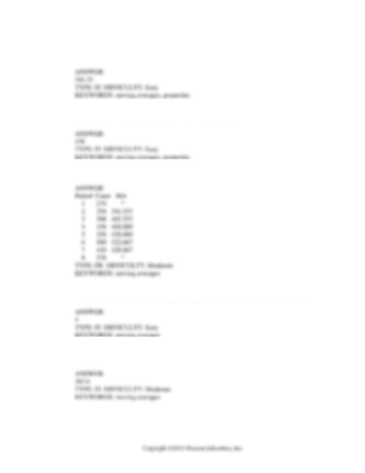
58. Referring to Scenario 16-4, construct a centered 3-year moving average for the wine sales.
59. Referring to Scenario 16-4, a centered 5-year moving average is to be constructed for the
wine sales. The number of moving averages that will be calculated is __________.
60. Referring to Scenario 16-4, a centered 5-year moving average is to be constructed for the
wine sales. The moving average for 2007 is __________.
16-18 Time-Series Forecasting
61. Referring to Scenario 16-4, a centered 5-year moving average is to be constructed for the
wine sales. The moving average for 2010 is __________.
62. Referring to Scenario 16-4, construct a centered 5-year moving average for the wine sales.
63. Referring to Scenario 16-4, exponential smoothing with a weight or smoothing constant of
0.2 will be used to smooth the wine sales. The value of E2, the smoothed value for 2006 is
__________.
64. Referring to Scenario 16-4, exponential smoothing with a weight or smoothing constant of
0.2 will be used to smooth the wine sales. The value of E4, the smoothed value for 2008 is
__________.
65. Referring to Scenario 16-4, exponential smoothing with a weight or smoothing constant of
0.2 will be used to forecast wine sales. The forecast for 2013 is __________.
Time-Series Forecasting 16-19
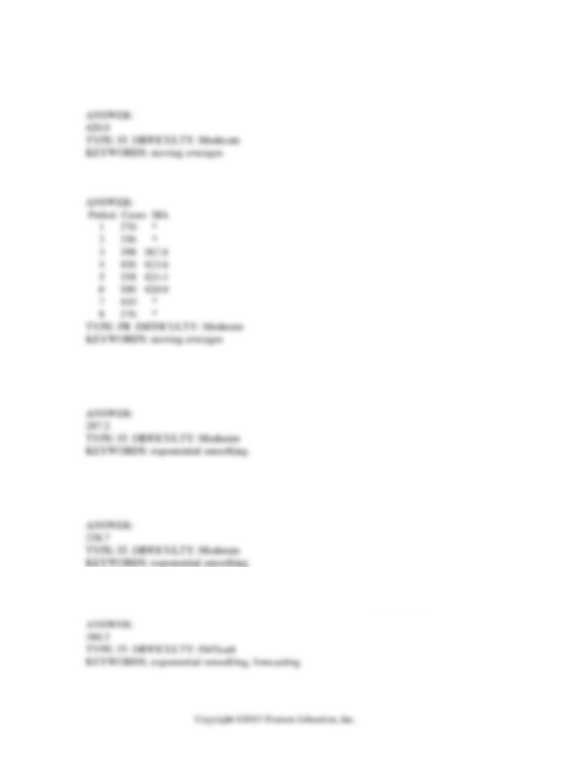
66. Referring to Scenario 16-4, exponentially smooth the wine sales with a weight or smoothing
constant of 0.2.
67. Referring to Scenario 16-4, exponential smoothing with a weight or smoothing constant of
0.4 will be used to smooth the wine sales. The value of E2, the smoothed value for 2006 is
__________.
68. Referring to Scenario 16-4, exponential smoothing with a weight or smoothing constant of
0.4 will be used to smooth the wine sales. The value of E5, the smoothed value for 2009 is
__________.
KEYWORDS: exponential smoothing
69. Referring to Scenario 16-4, exponential smoothing with a weight or smoothing constant of
0.4 will be used to forecast wine sales. The forecast for 2013 is __________.
16-20 Time-Series Forecasting
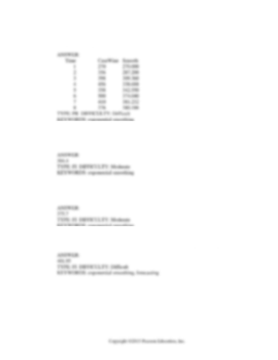
70. Referring to Scenario 16-4, exponentially smooth the wine sales with a weight or smoothing
constant of 0.4.
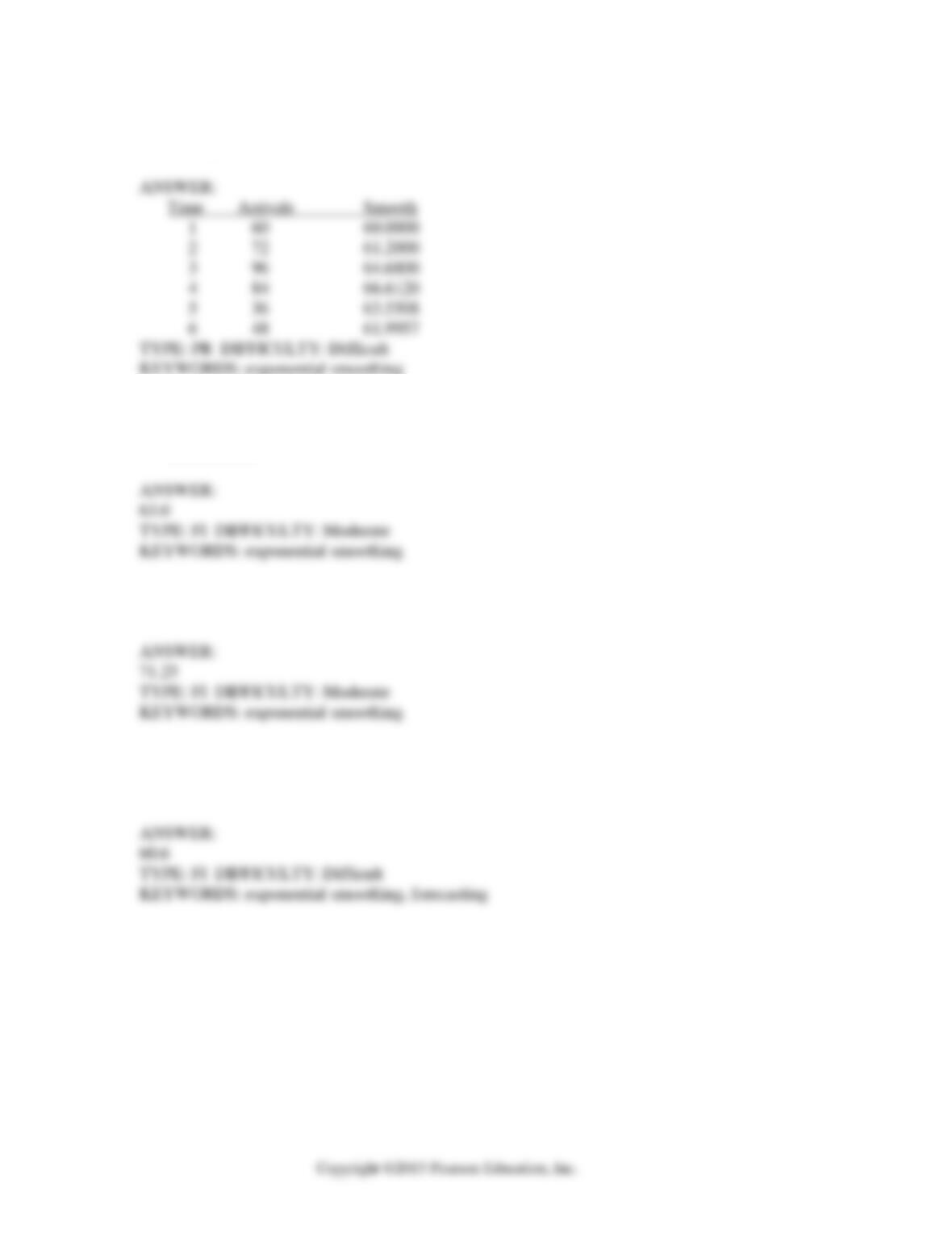
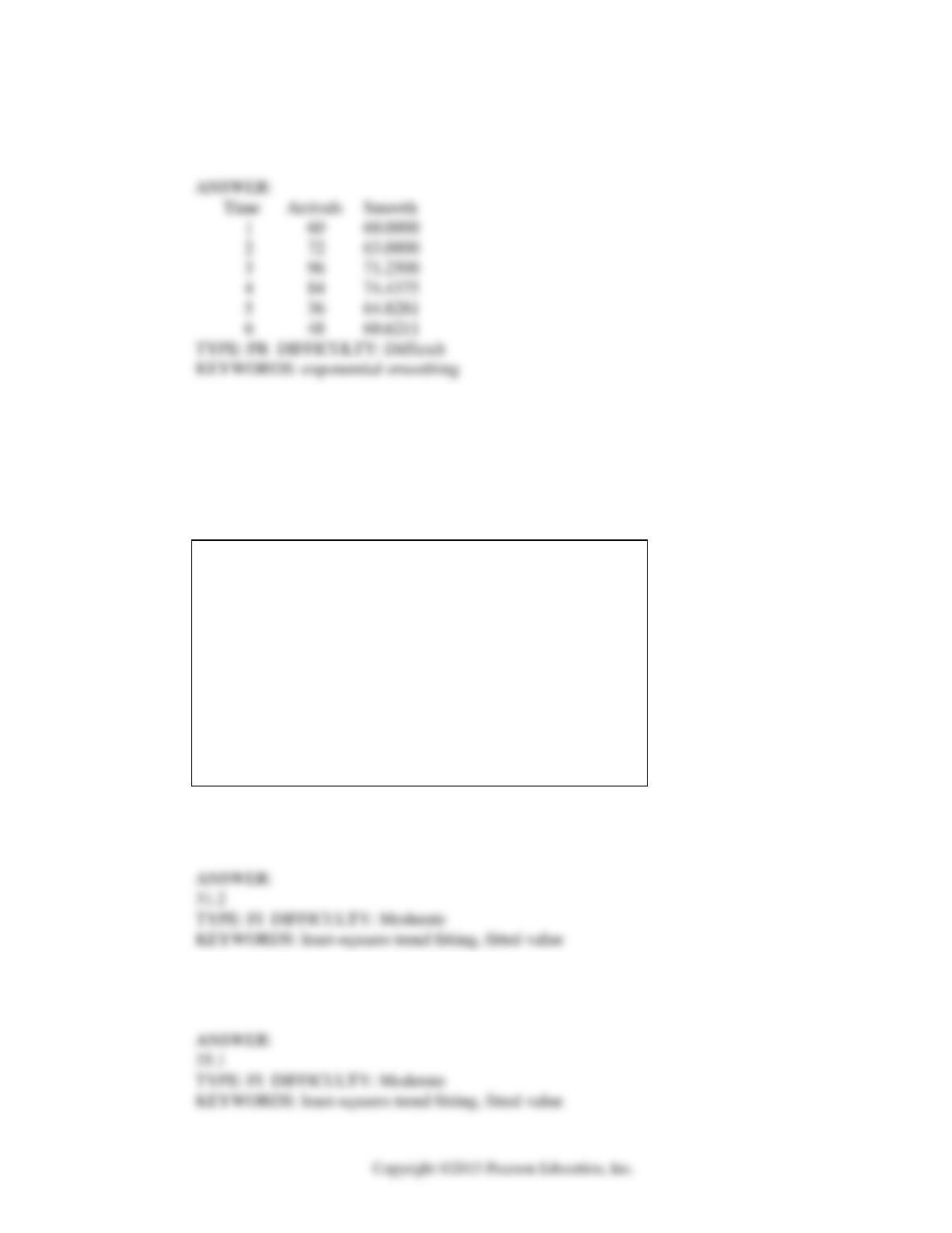
SCENARIO 16-5
The number of passengers arriving at San Francisco on the Amtrak cross-country express on 6
successive Mondays were: 60, 72, 96, 84, 36, and 48.
71. Referring to Scenario 16-5, the number of arrivals will be smoothed with a 3-term moving
average. There will be a total of __________ smoothed values.
72. Referring to Scenario 16-5, the number of arrivals will be smoothed with a 3-term moving
average. The first smoothed value will be __________.
73. Referring to Scenario 16-5, the number of arrivals will be smoothed with a 3-term moving
average. The last smoothed value will be __________.
Time-Series Forecasting 16-21
74. Referring to Scenario 16-5, the number of arrivals will be smoothed with a 5-term moving
average. The first smoothed value will be __________.
75. Referring to Scenario 16-5, the number of arrivals will be smoothed with a 5-term moving
average. The last smoothed value will be __________.
76. Referring to Scenario 16-5, the number of arrivals will be exponentially smoothed with a
smoothing constant of 0.1. The smoothed value for the second Monday will be __________.
77. Referring to Scenario 16-5, the number of arrivals will be exponentially smoothed with a
smoothing constant of 0.1. The smoothed value for the sixth Monday will be __________.
78. Referring to Scenario 16-5, the number of arrivals will be exponentially smoothed with a
smoothing constant of 0.1. Then the forecast for the seventh Monday will be __________.
16-22 Time-Series Forecasting
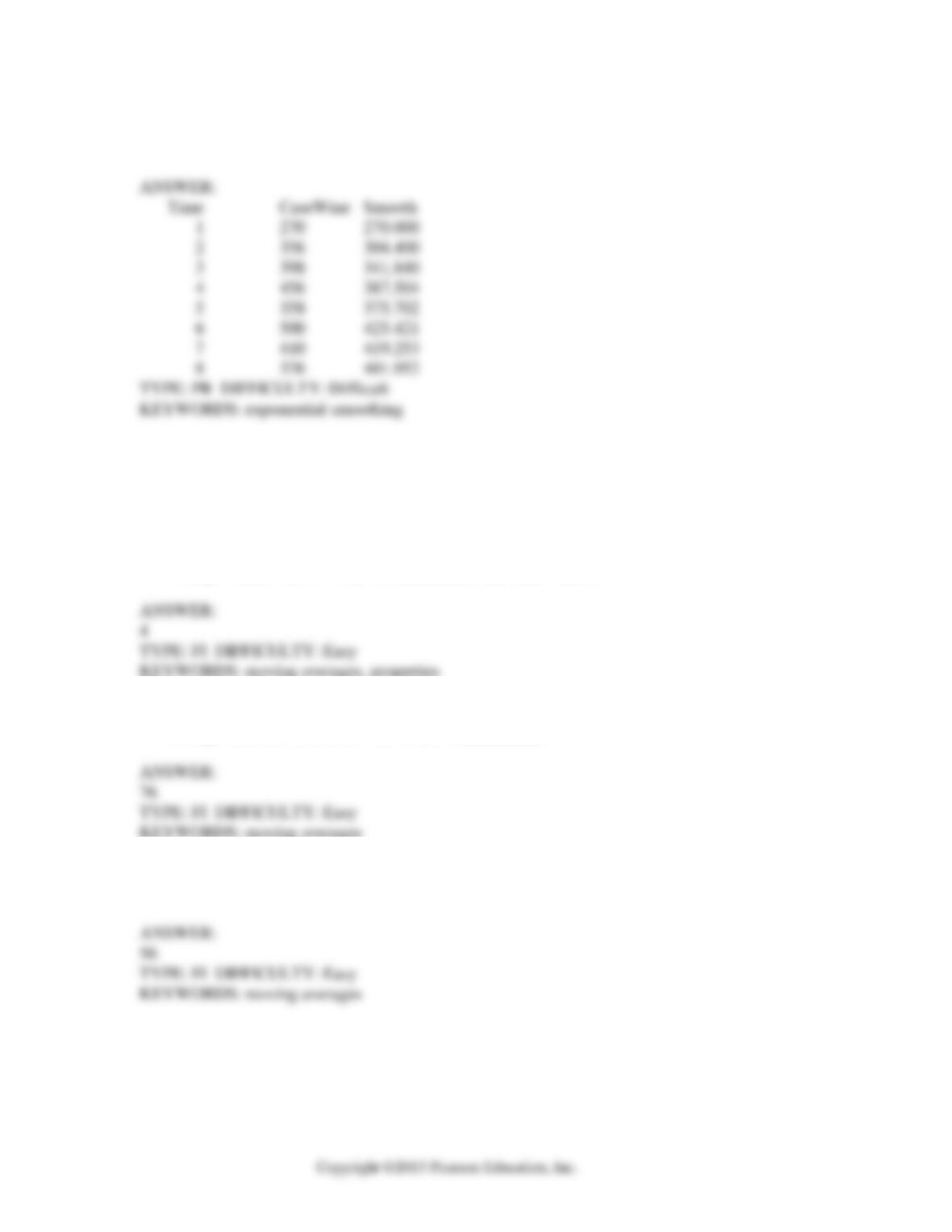
79. Referring to Scenario 16-5, exponentially smooth the number of arrivals using a smoothing
constant of 0.1.
80. Referring to Scenario 16-5, the number of arrivals will be exponentially smoothed with a
smoothing constant of 0.25. The smoothed value for the second Monday will be
__________.
81. Referring to Scenario 16-5, the number of arrivals will be exponentially smoothed with a
smoothing constant of 0.25. The smoothed value for the third Monday will be __________.
82. Referring to Scenario 16-5, the number of arrivals will be exponentially smoothed with a
smoothing constant of 0.25. The forecast of the number of arrivals on the seventh Monday
will be __________.
Time-Series Forecasting 16-23
83. Referring to Scenario 16-5, exponentially smooth the number of arrivals using a smoothing
constant of 0.25.
SCENARIO 16-6
The president of a chain of department stores believes that her stores’ total sales have been
showing a linear trend since 1993. She uses Microsoft Excel to obtain the partial output below.
The dependent variable is sales (in millions of dollars), while the independent variable is coded
years, where 1993 is coded as 0, 1994 is coded as 1, etc.
SUMMARY OUTPUT
Regression Statistics
Multiple R 0.604
R Square 0.365
Adjusted R Square 0.316
Standard Error 4.800
Observations 17
Coefficients
Intercept 31.2
Coded Year 0.78
84. Referring to Scenario 16-6, the fitted trend value (in millions of dollars) for 1993 is
__________.
85. Referring to Scenario 16-6, the fitted trend value (in millions of dollars) for 1998 is
__________.
16-24 Time-Series Forecasting
86. Referring to Scenario 16-6, the estimate of the amount by which sales (in millions of dollars)
is increasing each year is __________.
__________.
88. Referring to Scenario 16-6, the forecast for sales (in millions of dollars) in 2015 is
__________.
SCENARIO 16-7
The executive vice-president of a drug manufacturing firm believes that the demand for the firm’s
most popular drug has been evidencing an exponential trend since 1999. She uses Microsoft
Excel to obtain the partial output below. The dependent variable is the log base 10 of the demand
for the drug, while the independent variable is years, where 1999 is coded as 0, 2000 is coded as
1, etc.
SUMMARY OUTPUT
Regression Statistics
Multiple R 0.996
R Square 0.992
Adjusted R Square 0.991
Standard Error 0.02831
Observations 12
Coefficients
Intercept 1.44
Coded Year 0.068
Time-Series Forecasting 16-25
89. Referring to Scenario 16-7, the fitted trend value for 1999 is __________.
90. Referring to Scenario 16-7, the fitted trend value for 2004 is __________.
91. Referring to Scenario 16-7, the fitted exponential trend equation to predict Y is __________.
92. Referring to Scenario 16-7, the forecast for the demand in 2013 is __________.
93. Referring to Scenario 16-7, the forecast for the demand in 2016 is __________.
16-26 Time-Series Forecasting
SCENARIO 16-8
The manager of a marketing consulting firm has been examining his company’s yearly profits. He
believes that these profits have been showing a quadratic trend since 1994. He uses Microsoft
Excel to obtain the partial output below. The dependent variable is profit (in thousands of
dollars), while the independent variables are coded years and squared of coded years, where 1994
is coded as 0, 1995 is coded as 1, etc.
SUMMARY OUTPUT
Regression Statistics
Multiple R 0.998
R Square 0.996
Adjusted R Square 0.996
Standard Error 4.996
Observations 17
Coefficients
Intercept 35.5
Coded Year 0.45
Year Squared 1.00
94. Referring to Scenario 16-8, the fitted value for 1994 is __________.
95. Referring to Scenario 16-8, the fitted value for 1999 is __________.
96. Referring to Scenario 16-8, the forecast for profits in 2014 is __________.
97. Referring to Scenario 16-8, the forecast for profits in 2019 is __________.
Time-Series Forecasting 16-27
SCENARIO 16-9
Given below are EXCEL outputs for various estimated autoregressive models for a company’s
real operating revenues (in billions of dollars) from 1989 to 2012. From the data, you also know
that the real operating revenues for 2010, 2011, and 2012 are 11.7909, 11.7757 and 11.5537,
respectively.
First-Order Autoregressive Model:
Coefficients
Standard Error
t Stat
P-value
Intercept
0.1802
0.3980
0.4528
0.6553
XLag1
1.0112
0.0497
20.3526
0.0000
Second-Order Autoregressive Model:
Coefficients
Standard Error
t Stat
P-value
Intercept
0.3005
0.4408
0.6817
0.5036
X Lag 1
1.1732
0.2347
4.9980
0.0001
X Lag 2
-0.1830
0.2507
-0.7300
0.4743
Third-Order Autoregressive Model:
Coefficients
Standard Error
t Stat
P-value
Intercept
0.3130
0.5144
0.6085
0.5509
XLag1
1.1737
0.2465
4.7617
0.0002
XLag2
-0.0694
0.3731
-0.1860
0.8547
XLag3
-0.1221
0.2820
-0.4330
0.6704
98. Referring to Scenario 16-9 and using a 5% level of significance, what is the appropriate
autoregressive model for the company’s real operating revenue?
a) First-Order Autoregressive Model
b) Second-Order Autoregressive
c) Third-Order Autoregressive
d) Any of the above
16-28 Time-Series Forecasting
99. Referring to Scenario 16-9, if one decides to use the Third-Order Autoregressive model ,
what will the predicted real operating revenue for the company be in 2013?
a) $11.55 billion
b) $11.62 billion
c) $11.84 billion
d) $12.47 billion
100. Referring to Scenario 16-9, if one decides to use the Third-Order Autoregressive model ,
what will the predicted real operating revenue for the company be in 2014?
a) $11.55 billion
b) $11.62 billion
c) $12.47 billion
d) $12.57 billion
101. Referring to Scenario 16-9, if one decides to use the Third-Order Autoregressive model ,
what will the predicted real operating revenue for the company be in 2015?
a) $11.59 billion
b) $11.68 billion
c) $11.84 billion
d) $12.47 billion
Time-Series Forecasting 16-29
SCENARIO 16-10
Business closures in a city in the western U.S. from 2007 to 2012 were:
2007 10
2008 11
2009 13
2010 19
2011 24
2012 35
Microsoft Excel was used to fit both first-order and second-order autoregressive models,
resulting in the following partial outputs:
SUMMARY OUTPUT – 2nd Order Model
Coefficients
Intercept -5.77
X Variable 1 0.80
X Variable 2 1.14
SUMMARY OUTPUT – 1st Order Model
Coefficients
Intercept -4.16
X Variable 1 1.59
102. Referring to Scenario 16-10, the fitted values for the first-order autoregressive model are
________, ________, ________, ________, and ________.
103. Referring to Scenario 16-10, the residuals for the first-order autoregressive model are
________, ________, ________, ________, and ________.
104. Referring to Scenario 16-10, the value of the MAD for the first-order autoregressive model
is ________.
16-30 Time-Series Forecasting
105. Referring to Scenario 16-10, the fitted values for the second-order autoregressive model
are ________, ________, ________, and ________.
106. Referring to Scenario 16-10, the residuals for the second-order autoregressive model are
________, ________, ________, and ________.
107. Referring to Scenario 16-10, the value of the MAD for the second-order autoregressive
model is ________.
108. True or False: Referring to Scenario 16-10, the values of the MAD for the two models
indicate that the first-order model should be used for forecasting.

Time-Series Forecasting 16-31
SCENARIO 16-11
The manager of a health club has recorded mean attendance in newly introduced step classes
over the last 15 months: 32.1, 39.5, 40.3, 46.0, 65.2, 73.1, 83.7, 106.8, 118.0, 133.1, 163.3, 182.8,
205.6, 249.1, and 263.5. She then used Microsoft Excel to obtain the following partial output for
both a first– and second-order autoregressive model.
SUMMARY OUTPUT – 2nd Order Model
Regression Statistics
Multiple R 0.993
R Square 0.987
Adjusted R Square 0.985
Standard Error 9.276
Observations 15
Coefficients
Intercept 5.86
X Variable 1 0.37
X Variable 2 0.85
SUMMARY OUTPUT – 1st Order Model
Regression Statistics
Multiple R 0.993
R Square 0.987
Adjusted R Square 0.985
Standard Error 9.150
Observations 15
Coefficients
Intercept 5.66
X Variable 1 1.10
109. Referring to Scenario 16-11, using the first-order model, the forecast of mean attendance
for month 16 is __________.
ANSWER:

16-32 Time-Series Forecasting
110. Referring to Scenario 16-11, using the first-order model, the forecast of mean attendance
for month 17 is __________.
111. Referring to Scenario 16-11, using the second-order model, the forecast of mean
attendance for month 16 is __________.
ANSWER:
112. Referring to Scenario 16-11, using the second-order model, the forecast of mean
attendance for month 17 is __________.
113. True or False: Referring to Scenario 16-11, based on the parsimony principle, the second–
order model is the better model for making forecasts.
SCENARIO 16-12
A local store developed a multiplicative time-series model to forecast its revenues in future
quarters, using quarterly data on its revenues during the 5-year period from 2009 to 2013. The
following is the resulting regression equation:
Y
ˆ
log 10
= 6.102 + 0.012 X – 0.129 Q1 – 0.054 Q2 + 0.098 Q3
where
Y
ˆ
is the estimated number of contracts in a quarter
X is the coded quarterly value with X = 0 in the first quarter of 2008.
Q1 is a dummy variable equal to 1 in the first quarter of a year and 0 otherwise.
Q2 is a dummy variable equal to 1 in the second quarter of a year and 0 otherwise.
Q3 is a dummy variable equal to 1 in the third quarter of a year and 0 otherwise.
Time-Series Forecasting 16-33
114. Referring to Scenario 16-12, the best interpretation of the constant 6.102 in the regression
equation is:
a) the fitted value for the first quarter of 2009, prior to seasonal adjustment, is
log10(6.102).
b) the fitted value for the first quarter of 2009, after to seasonal adjustment, is
log10(6.102).
c) the fitted value for the first quarter of 2009, prior to seasonal adjustment, is 106.102.
d) the fitted value for the first quarter of 2009, after to seasonal adjustment, is 106.102.
115. Referring to Scenario 16-12, the best interpretation of the coefficient of X (0.012) in the
regression equation is:
a) the quarterly compound growth rate in revenues is around 2.8%.
b) the annual growth rate in revenues is around 2.8%.
c) the quarterly growth rate in revenues is around 1.2%.
d) the annual growth rate in revenues is around 1.2%.
116. Referring to Scenario 16-12, the estimated quarterly compound growth rate in revenues is
around:
a) 1.2%.
b) 2.8%.
c) 12%.
d) 28%.
16-34 Time-Series Forecasting
117. Referring to Scenario 16-12, the best interpretation of the coefficient of Q2 (–0.054) in the
regression equation is:
a) the revenues in the second quarter of a year is approximately 5.4% lower than the
average over all 4 quarters.
b) the revenues in the second quarter of a year is approximately 5.4% lower than it
would be during the fourth quarter.
c) the revenues in the second quarter of a year is approximately 11.69% lower than the
average over all 4 quarters.
d) the revenues in the second quarter of a year is approximately 11.69% lower than it
would be during the fourth quarter.
118. Referring to Scenario 16-12, the best interpretation of the coefficient of Q3 (0.098) in the
regression equation is:
a) the revenues in the third quarter of a year is approximately 9.8% higher than the
average over all 4 quarters.
b) the revenues in the third quarter of a year is approximately 9.8% higher than it would
be during the fourth quarter.
c) the revenues in the third quarter of a year is approximately 25.31% higher than the
average over all 4 quarters.
d) the revenues in the third quarter of a year is approximately 25.31% higher than it
would be during the fourth quarter.
119. Referring to Scenario 16-12, to obtain the fitted value for the first quarter of 2013 using the
model, which of the following sets of values should be used in the regression equation?
a) X = 16, Q1 = 1, Q2 = 0, Q3 = 0
b) X = 16, Q1 = 0, Q2 = 1, Q3 = 0
c) X = 17, Q1 = 1, Q2 = 0, Q3 = 0
d) X = 17, Q1 = 0, Q2 = 1, Q3 = 0
Time-Series Forecasting 16-35
120. Referring to Scenario 16-12, to obtain a fitted value for the fourth quarter of 2010 using the
model, which of the following sets of values should be used in the regression equation?
a) X = 7, Q1 = 0, Q2 = 0, Q3 = 0
b) X = 7, Q1 = 1, Q2 = 0, Q3 = 0
c) X = 8, Q1 = 0, Q2 = 0, Q3 = 0
d) X = 8, Q1 = 1, Q2 = 0, Q3 = 0
121. Referring to Scenario 16-12, to obtain a forecast for the third quarter of 2014 using the
model, which of the following sets of values should be used in the regression equation?
a) X = 22, Q1 = 0, Q2 = 0, Q3 = 0
b) X = 22, Q1 = 0, Q2 = 0, Q3 = 1
c) X = 23, Q1 = 0, Q2 = 0, Q3 = 0
d) X = 23, Q1 = 0, Q2 = 0, Q3 = 1
122. Referring to Scenario 16-12, using the regression equation, what is the forecast for the
revenues in the third quarter of 2014?
123. Referring to Scenario 16-12, using the regression equation, what is the forecast for the
revenues in the first quarter of 2016?
124. Referring to Scenario 16-12, using the regression equation, what is the forecast for the
revenues in the fourth quarter of 2015?
16-36 Time-Series Forecasting
125. Referring to Scenario 16-12, in testing the significance of the coefficient of X in the
regression equation (0.012) which has a p-value of 0.0000. Which of the following is the best
interpretation of this result?
a) The quarterly growth rate in revenues is significantly different from 0% (
= 0.05).
b) The quarterly growth rate in revenues is not significantly different from 0% (
=
0.05).
c) The quarterly growth rate in revenues is significantly different from 1.2% (
=
0.05).
d) The quarterly growth rate in revenues is not significantly different from 1.2% (
=
0.05).
126. Referring to Scenario 16-12, in testing the significance of the coefficient for Q1 in the
regression equation (– 0.129) which has a p-value of 0.492. Which of the following is the
best interpretation of this result?
a) The revenues in the first quarter of the year are significantly different from the
revenues in an average quarter (
= 0.05).
b) The revenues in the first quarter of the year are not significantly different from the
revenues in an average quarter (
= 0.05).
c) The revenues in the first quarter of the year are significantly different from the
revenues in the fourth quarter (
= 0.05).
d) The revenues in the first quarter of the year are not significantly different from the
revenues in the fourth quarter (
= 0.05).

Time-Series Forecasting 16-37
SCENARIO 16-13
Given below is the monthly time series data for U.S. retail sales of building materials over a
specific year.
Month
Retail Sales
1
6,594
2
6,610
3
8,174
4
9,513
5
10,595
6
10,415
7
9,949
8
9,810
9
9,637
10
9,732
11
9,214
12
9,201
The results of the linear trend, quadratic trend, exponential trend, first-order autoregressive,
second-order autoregressive and third-order autoregressive model are presented below in which
the coded month for the 1st month is 0:
Linear trend model:
Coefficients
Standard Error
t Stat
P-value
Intercept
7950.7564
617.6342
12.8729
0.0000
Coded Month
212.6503
95.1145
2.2357
0.0494
Quadratic trend model:
Coefficients
Standard Error
t Stat
P-value
Intercept
6358.2473
417.2692
15.2378
0.0000
Coded Month
1168.1558
176.3526
6.6240
0.0001
Coded Month^2
-86.8641
15.4474
-5.6232
0.0003
Exponential trend model:
Coefficients
Standard Error
t Stat
P-value
Intercept
3.8912
0.0315
123.3674
0.0000
Coded Month
0.0116
0.0049
2.3957
0.0376
First-order autoregressive:
Coefficients
Standard Error
t Stat
P-value
Intercept
3132.0951
1287.2899
2.4331
0.0378
YLag1
0.6823
0.1398
4.8812
0.0009
16-38 Time-Series Forecasting
Second-order autoregressive::
Coefficients
Standard Error
t Stat
P-value
Intercept
4968.5789
766.9416
6.4784
0.0003
YLag1
0.9333
0.1547
6.0316
0.0005
YLag2
-0.4487
0.1238
-3.6235
0.0085
Third-order autoregressive::
Coefficients
Standard Error
t Stat
P-value
Intercept
6782.7567
2105.7115
3.2211
0.0234
YLag1
0.5481
0.3918
1.3990
0.2207
YLag2
0.0198
0.4034
0.0490
0.9628
YLag3
-0.2749
0.2234
-1.2308
0.2731
Below is the residual plot of the various models:
–2000
–1500
–1000
–500
0
500
1000
1500
2000
2500
1
2
3
4
5
6
7
8
9
10
11
12
Residuals
Axis Title
Residual Plot
Linear-trend
Quadratic-trend
Exponential-trend
AR(1)
AR(2)
AR(3)
Time-Series Forecasting 16-39
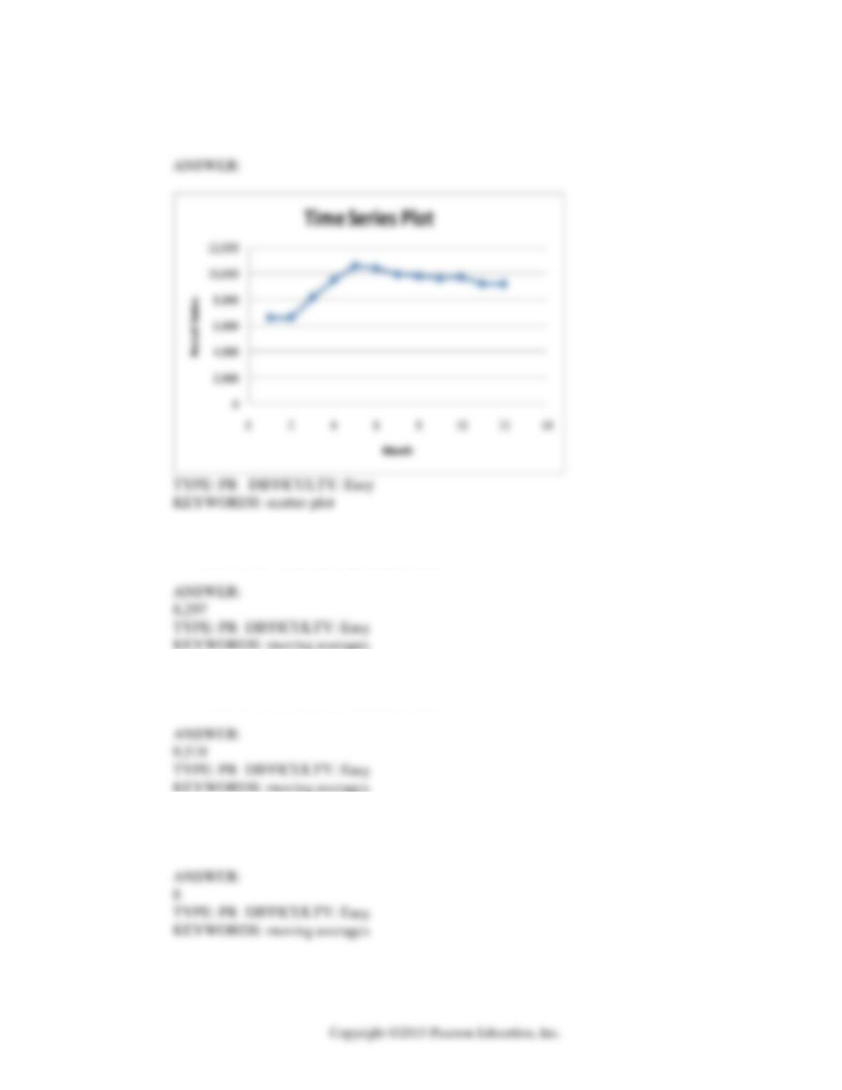
127. Referring to Scenario 16-13, construct a scatter plot (i.e., a time-series plot) with month on
the horizontal X-axis.
128. Referring to Scenario 16-13, if a five-month moving average is used to smooth this series,
what would be the first calculated value?
129. Referring to Scenario 16-13, if a five-month moving average is used to smooth this series,
what would be the last calculated value?
130. Referring to Scenario 16-13, if a five-month moving average is used to smooth this series,
how many moving averages can you compute?
16-40 Time-Series Forecasting
131. Referring to Scenario 16-13, what is the exponentially smoothed value for the first month
using a smoothing coefficient of W = 0.5?
132. Referring to Scenario 16-13, what is the exponentially smoothed value for the second
month using a smoothing coefficient of W = 0.5?
133. Referring to Scenario 16-13, what is the exponentially smoothed value for the 12th month
using a smoothing coefficient of W = 0.5 if the exponentially smooth value for the 10th and
11th month are 9,746.3672 and 9,480.1836, respectively?
134. Referring to Scenario 16-13, what is the exponentially smoothed forecast for the 13th
month using a smoothing coefficient of W = 0.5 if the exponentially smooth value for the 10th
and 11th month are 9,746.3672 and 9,480.1836, respectively?
135. Referring to Scenario 16-13, what is the exponentially smoothed value for the first month
using a smoothing coefficient of W = 0.25?
136. Referring to Scenario 16-13, what is the exponentially smoothed value for the second
month using a smoothing coefficient of W = 0.25?
Time-Series Forecasting 16-41
137. Referring to Scenario 16-13, what is the exponentially smoothed value for the 12th month
using a smoothing coefficient of W = 0.25 if the exponentially smooth value for the 10th and
11th month are 9,477.7776 and 9,411.8332, respectively?
138. Referring to Scenario 16-13, what is the exponentially smoothed forecast for the 13th
month using a smoothing coefficient of W = 0.25 if the exponentially smooth value for the
10th and 11th month are 9,477.7776 and 9,411.8332, respectively?
139. Referring to Scenario 16-13, what is your forecast for the 13th month using the linear-trend
model?
140. Referring to Scenario 16-13, what is the p-value for the t test statistic for testing the
significance of the quadratic term in the quadratic-trend model?
141. Referring to Scenario 16-13, what is the value of the t test statistic for testing the
significance of the quadratic term in the quadratic-trend model?
142. True or False: Referring to Scenario 16-13, you can conclude that the quadratic term in the
quadratic-trend model is statistically significant at the 5% level of significance.
16-42 Time-Series Forecasting
143. Referring to Scenario 16-13, what is your forecast for the 13th month using the quadratic-
trend model?
144. Referring to Scenario 16-13, what is your forecast for the 13th month using the exponential-
trend model?
145. Referring to Scenario 16-13, what is your estimated annual compound growth rate using
the exponential-trend model?
146. Referring to Scenario 16-13, what is the value of the t test statistic for testing the
appropriateness of the third-order autoregressive model?
147. Referring to Scenario 16-13, what is the p-value of the t test statistic for testing the
appropriateness of the third-order autoregressive model?
148. True or False: Referring to Scenario 16-13, you can reject the null hypothesis for testing
the appropriateness of the third-order autoregressive model at the 5% level of significance.
Time-Series Forecasting 16-43
149. True or False: Referring to Scenario 16-13, you can conclude that the third-order
autoregressive model is appropriate at the 5% level of significance.
150. Referring to Scenario 16-13, what is the value of the t test statistic for testing the
appropriateness of the second-order autoregressive model?
151. Referring to Scenario 16-13, what is the p-value of the t test statistic for testing the
appropriateness of the second-order autoregressive model?
152. True or False: Referring to Scenario 16-13, you can reject the null hypothesis for testing
the appropriateness of the second-order autoregressive model at the 5% level of significance.
153. True or False: Referring to Scenario 16-13, you can conclude that the second-order
autoregressive model is appropriate at the 5% level of significance.
16-44 Time-Series Forecasting
154. Referring to Scenario 16-13, the best autoregressive model using the 5% level of
significance is
a) first-order
b) second-order
c) third-order
d) none of the above
155. Referring to Scenario 16-13, what is your forecast for the 13th month using the first-order
autoregressive model?
156. Referring to Scenario 16-13, what is your forecast for the 13th month using the second-
order autoregressive model?
157. Referring to Scenario 16-13, what is your forecast for the 13th month using the third-order
autoregressive model?
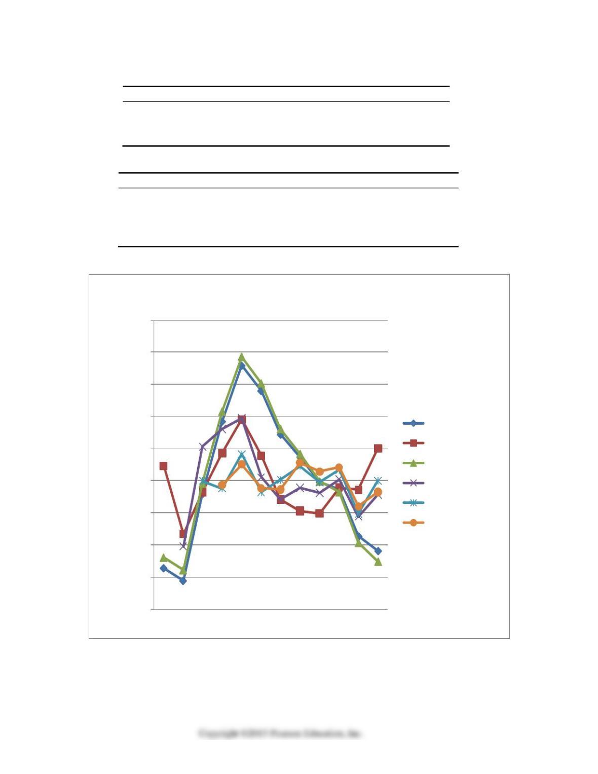
158. True or False: Referring to Scenario 16-13, the best model based on the residual plots is
the linear-trend model.
Time-Series Forecasting 16-45
159. True or False: Referring to Scenario 16-13, the best model based on the residual plots is
the quadratic-trend regression model.
160. True or False: Referring to Scenario 16-13, the best model based on the residual plots is
the exponential-trend regression model.
161. True or False: Referring to Scenario 16-13, the best model based on the residual plots is
the second-order autoregressive model.
SCENARIO 16-14
A contractor developed a multiplicative time-series model to forecast the number of contracts in
future quarters, using quarterly data on number of contracts during the 3-year period from 2011
to 2013. The following is the resulting regression equation:
ln
Y
ˆ
= 3.37 + 0.117 X – 0.083 Q1 + 1.28 Q2 + 0.617 Q3
where
Y
ˆ
is the estimated number of contracts in a quarter
X is the coded quarterly value with X = 0 in the first quarter of 2011.
Q1 is a dummy variable equal to 1 in the first quarter of a year and 0 otherwise.
Q2 is a dummy variable equal to 1 in the second quarter of a year and 0 otherwise.
Q3 is a dummy variable equal to 1 in the third quarter of a year and 0 otherwise.
162. Referring to Scenario 16-14 , the best interpretation of the constant 3.37 in the regression
equation is:
a) the fitted value for the first quarter of 2011, prior to seasonal adjustment, is log10
3.37.
b) the fitted value for the first quarter of 2011, after to seasonal adjustment, is log10
3.37.
c) the fitted value for the first quarter of 2011, prior to seasonal adjustment, is 103.37.
d) the fitted value for the first quarter of 2011, after to seasonal adjustment, is 103.37.
16-46 Time-Series Forecasting
163. Referring to Scenario 16-14, the best interpretation of the coefficient of X (0.117) in the
regression equation is:
a) the quarterly compound growth rate in contracts is around 30.92%.
b) the annually compound growth rate in contracts is around 30.92%.
c) the quarterly compound growth rate in contracts is around 11.7%.
d) the annually compound growth rate in contracts is around 11.7%.
164. Referring to Scenario 16-14, the best interpretation of the coefficient of Q3 (0.617) in the
regression equation is:
a) the number of contracts in the third quarter of a year is approximately 62% higher
than the average over all 4 quarters.
b) the number of contracts in the third quarter of a year is approximately 62% higher
than it would be during the fourth quarter.
c) the number of contracts in the third quarter of a year is approximately 314% higher
than the average over all 4 quarters.
d) the number of contracts in the third quarter of a year is approximately 314% higher
than it would be during the fourth quarter.
165. Referring to Scenario 16-14, to obtain a forecast for the first quarter of 2014 using the
model, which of the following sets of values should be used in the regression equation?
a) X = 12, Q1 = 0, Q2 = 0, Q3 = 0
b) X = 12, Q1 = 1, Q2 = 0, Q3 = 0
c) X = 13, Q1 = 0, Q2 = 0, Q3 = 0
d) X = 13, Q1 = 1, Q2 = 0, Q3 = 0
Time-Series Forecasting 16-47
166. Referring to Scenario 16-14, to obtain a forecast for the fourth quarter of 2014 using the
model, which of the following sets of values should be used in the regression equation?
a) X = 15, Q1 = 0, Q2 = 0, Q3 = 0
b) X = 15, Q1 = 1, Q2 = 0, Q3 = 0
c) X = 16, Q1 = 0, Q2 = 0, Q3 = 0
d) X = 16, Q1 = 1, Q2 = 0, Q3 = 0
167. Referring to Scenario 16-14, using the regression equation, which of the following values
is the best forecast for the number of contracts in the third quarter of 2014?
a) 49,091
b) 133,352
c) 421,697
d) 1,482,518
168. Referring to Scenario 16-14, using the regression equation, which of the following values
is the best forecast for the number of contracts in the second quarter of 2015?
a) 144,212
b) 391,742
c) 1,238,797
d) 4,355,119
16-48 Time-Series Forecasting
169. Referring to Scenario 16-14, in testing the coefficient of X in the regression equation
(0.117) the results were a t-statistic of 9.08 and an associated p-value of 0.0000. Which of
the following is the best interpretation of this result?
a) The quarterly growth rate in the number of contracts is significantly different from
0% (
= 0.05).
b) The quarterly growth rate in the number of contracts is not significantly different
from 0% (
= 0.05).
c) The quarterly growth rate in the number of contracts is significantly different from
100% (
= 0.05).
d) The quarterly growth rate in the number of contracts is not significantly different
from 100% (
= 0.05).
170. Referring to Scenario 16-14, in testing the coefficient for Q1 in the regression equation (–
0.083), the results were a t-statistic of – 0.66 and an associated p-value of 0.530. Which of
the following is the best interpretation of this result?
a) The number of contracts in the first quarter of the year is significantly different from
the number of contracts in an average quarter (
= 0.05).
b) The number of contracts in the first quarter of the year is not significantly different
from the number of contracts in an average quarter (
= 0.05).
c) The number of contracts in the first quarter of the year is significantly different from
the number of contracts in the fourth quarter for a given coded quarterly value of X
(
= 0.05).
d) The number of contracts in the first quarter of the year is not significantly different
from the number of contracts in the fourth quarter for a given coded quarterly value
of X (
= 0.05).