
IVA-2 Part IV: Models for Decision Making
Business Statistics: Part IV Name___________________
Models for Decision Making – Test A
Chapter 14: Interpret or analyze linear models or relationships.
1. Data are collected on the number of foreign visitors to a country (million) and total
tourism revenue ($billion) for a sample of 10 countries. According to the following
output, what is standard error of the slope for this estimated regression equation?
Regression Analysis: Tourism ($bill) versus Visitors (mill)
The regression equation is: Tourism ($bill) = 21.5 + 0.295 Visitors (mill)
Predictor Coef SE Coef
Constant 21.464 3.462
Visitors (mill) 0.29497 0.07917
S = 2.58307 R-Sq = 63.4%
A. 2.58307
B. 3.462
C. 0.07917
D. 6.672
E. 0.29497
Chapter 14: Interpret or analyze linear models or relationships.
2. According to the partial regression analysis output below, what is the t-statistic to test
whether the regression slope is significant?
Regression Analysis: Tourism ($bill) versus Visitors (mill)
The regression equation is: Tourism ($bill) = 21.5 + 0.295 Visitors (mill)
Predictor Coef SE Coef
Constant 21.464 3.462
Visitors (mill) 0.29497 0.07917
S = 2.58307 R-Sq = 63.4%
A. 6.20
B. 13.88
C. 0.07917
D. 2.58307
E. 3.73

Test A IVA-3
Chapter 14: Interpret or analyze linear models or relationships.
3. In a regression analysis predicting tourism revenue ($billion) using number of foreign
visitors (million), the P-value for the calculated test statistic is 0.006. At the 0.05
level of significance we
A. reject the null hypothesis.
B. do not reject the null hypothesis.
C. conclude that the number of foreign visitors is significant in explaining tourism
revenue.
D. Both A and C.
E. Both B and C.
Chapter 14: Interpret or analyze linear models or relationships.
4. According to the regression analysis output below, how much of the variability in
tourism revenue is accounted for by the number of foreign visitors?
Regression Analysis: Tourism ($bill) versus Visitors (mill)
The regression equation is: Tourism ($ bill) = 21.5 + 0.295 Visitors (mill)
Predictor Coef SE Coef
Constant 21.464 3.462
Visitors (mill) 0.29497 0.07917
S = 2.58307 R-Sq = 63.4%
A. 63.4 %
B. 13.8 %
C. 2.58 billion $
D. 21.464 %
E. 3.73 billion $
Chapter 14: Create, interpret, and apply confidence and prediction intervals.
5. If we were interested in using regression methods to predict the tourism revenue for a
particular country that had 30 million foreign visitors we should
A. construct a confidence interval using the regression equation.
B. construct a predication interval using the regression equation.
C. use the correlation.
D. use the standard error.
E. None of these.
IVA-4 Part IV: Models for Decision Making
Chapter 14: Interpret or analyze linear models or relationships.
6. Which of the following statements about a residual plot is true?
A. A curved pattern indicates nonlinear association between the variables.
B. A pattern of increasing spread indicates the predicted values become less reliable
as the explanatory variable increases.
C. If all of the residuals are very small, the model will predict accurately.
D. It should not be used if the regression results are not significant.
E. It cannot be used to analyze linear association.
Chapter 14: Interpret or analyze linear models or relationships.
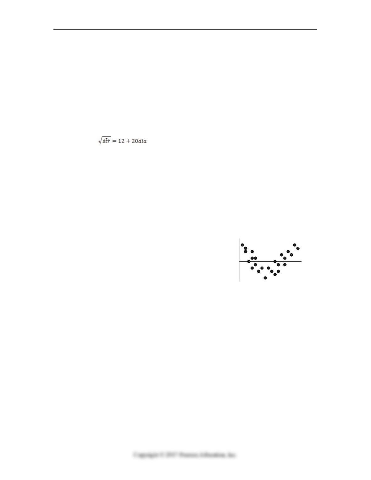
7. The model can be used to predict the breaking strength (pounds) of a
rope from its diameter (inches). According to this model, how much force should a
rope one-half inch in diameter withstand?
A. 484 pounds
B. 16 pounds
C. 22 pounds
D. 256 pounds
E. 4.7 pounds
Chapter 14: Determine when linear models are appropriate and/or useful for predicting
y-values.
8. According to the residual plot for a linear regression
model shown to the right, the linear model
A. okay because the same number of points is above the
line as below it.
B. okay because the association between the two
variables is fairly strong.
C. no good because the correlation is near 0.
D. no good because some residuals are large.
E. no good because of the curve in the residuals.

Test A IVA-5
Chapter 14: Interpret or analyze linear models or relationships.
9. Using the following regression analysis of the relationship between the size of cash
bonuses and pay scale, find the correlation between average annual cash bonus and
average annual pay?
Regression Analysis: Cash Bonus versus Pay
The regression equation is: Cash Bonus = – 4877 + 0.245 Pay
Predictor Coef SE Coef T P
Constant -4877 9106 -0.54 0.599
Pay 0.2453 0.1079 2.27 0.036
S = 13188.6 R-Sq = 22.3%
A. -0.540
B. -0.223
C. 0.108
D. 0.472
E. Cannot be determined from the information given.
Chapter 14: Interpret or analyze linear models or relationships.
10. According to the following regression analysis, the correlation between average
annual cash bonus and average annual pay using α = 0.05 is
Regression Analysis: Cash Bonus versus Pay
The regression equation is: Cash Bonus = – 4877 + 0.245 Pay
Predictor Coef SE Coef T P
Constant -4877 9106 -0.54 0.599
Pay 0.2453 0.1079 2.27 0.036
S = 13188.6 R-Sq = 22.3%
A. not significantly different from zero.
B. negative but not significantly different from zero.
C. positive and significantly different from zero.
D. negative and significantly different from zero.
E. Cannot be determined from the information given.
IVA-6 Part IV: Models for Decision Making
Chapter 14: Determine when linear models are appropriate and/or useful for predicting
y-values.
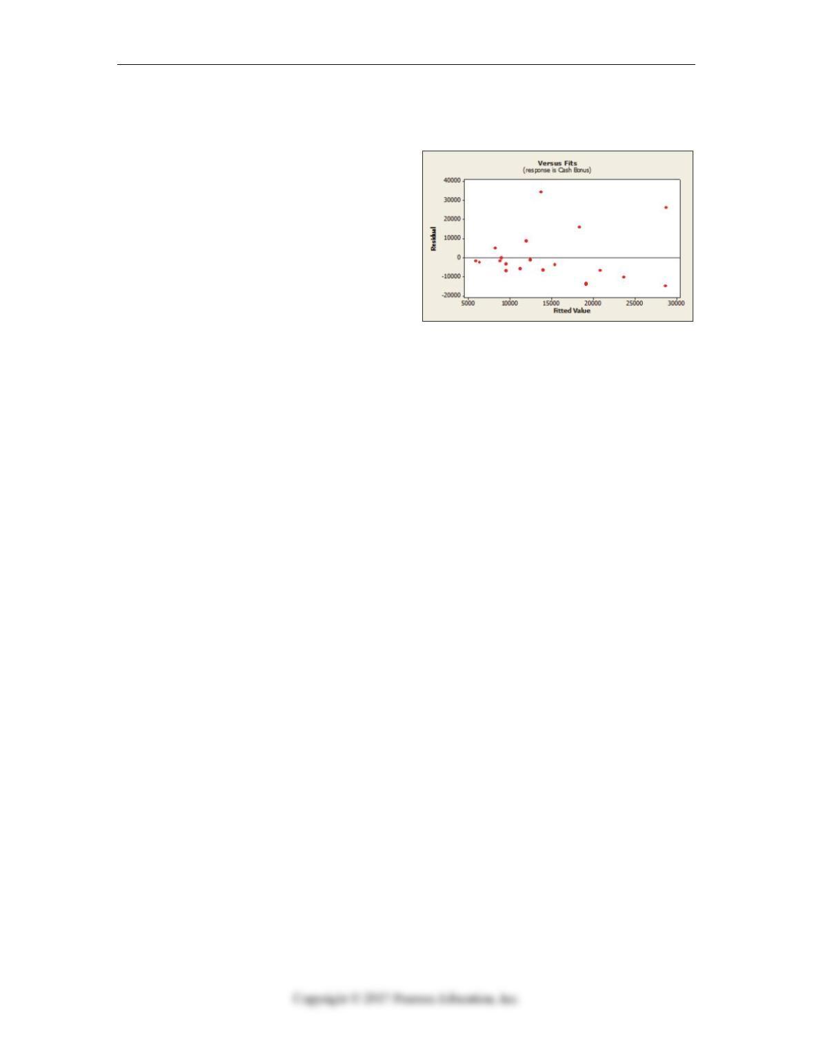
11. From its plot of residuals versus fitted
values shown below, which assumption
appears to be violated?
A. Equal Variance
B. Linearity
C. Normality
D. Independence
E. None; all appear to be satisfied.
Chapter 14: Determine when linear models are appropriate and/or useful for predicting
y-values.
12. Based on the regression output shown below, which of the following statements is
true?
The regression equation is
Price (cents) = 128 + 1.08 Time
Predictor Coef SE Coef T P
Constant 128.112 2.092 61.25 0.000
Time 1.0782 0.1407 7.66 0.000
S = 5.07299 R-Sq = 71.9%
Durbin-Watson statistic = 0.244822
A. The regression slope is significantly different from zero.
B. The model explains 71.9% of the variability in heating oil prices.
C. The linear model is appropriate.
D. Both A and B.
E. All of the above.
Test A IVA-7
Chapter 14: Determine when linear models are appropriate and/or useful for predicting
y-values.
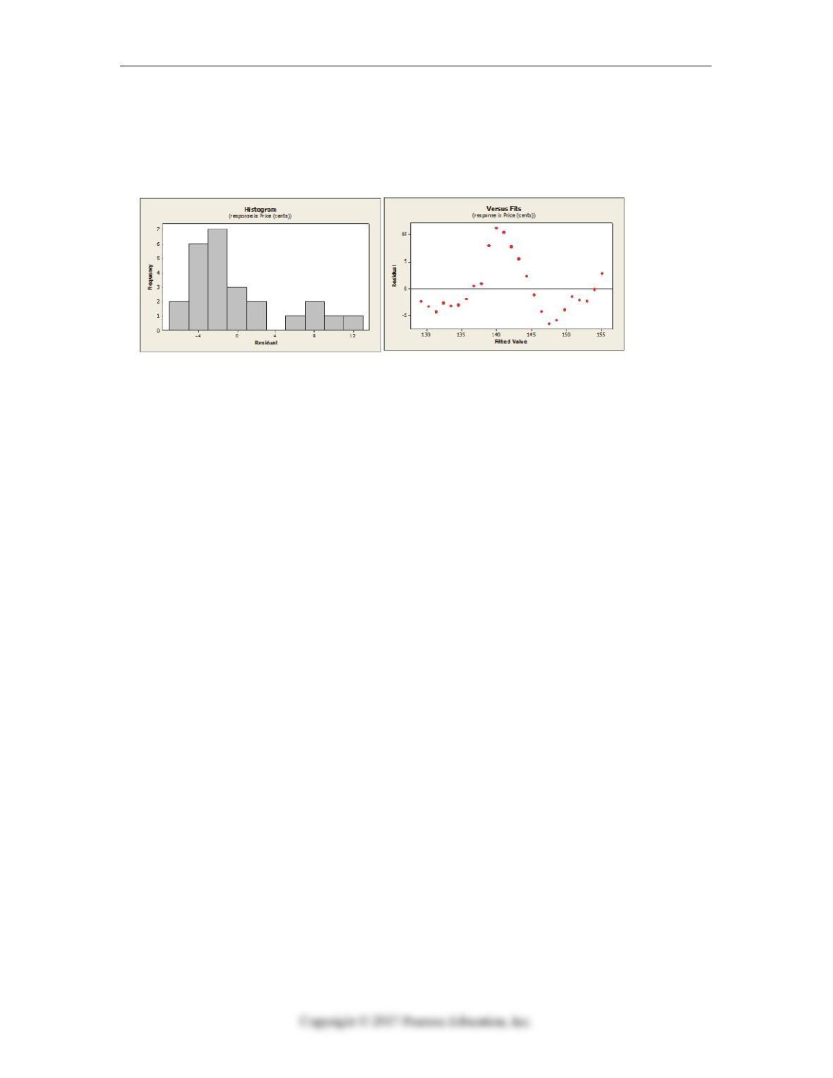
13. According to the residual plots shown below, which linear regression assumptions
appear to be violated?
A. Linearity
B. Normality
C. Equal Variance
D. Both A and B
E. All of the above
Chapter 16: Understand the data mining process.
14. Disparate databases that include demographic and transactional variables merged
together are referred to as
A. Data storage bins
B. Data mines
C. OLAP
D. CRISP
E. Data warehouses
IVA-8 Part IV: Models for Decision Making
Chapter 14: Determine if a re-expression is appropriate.
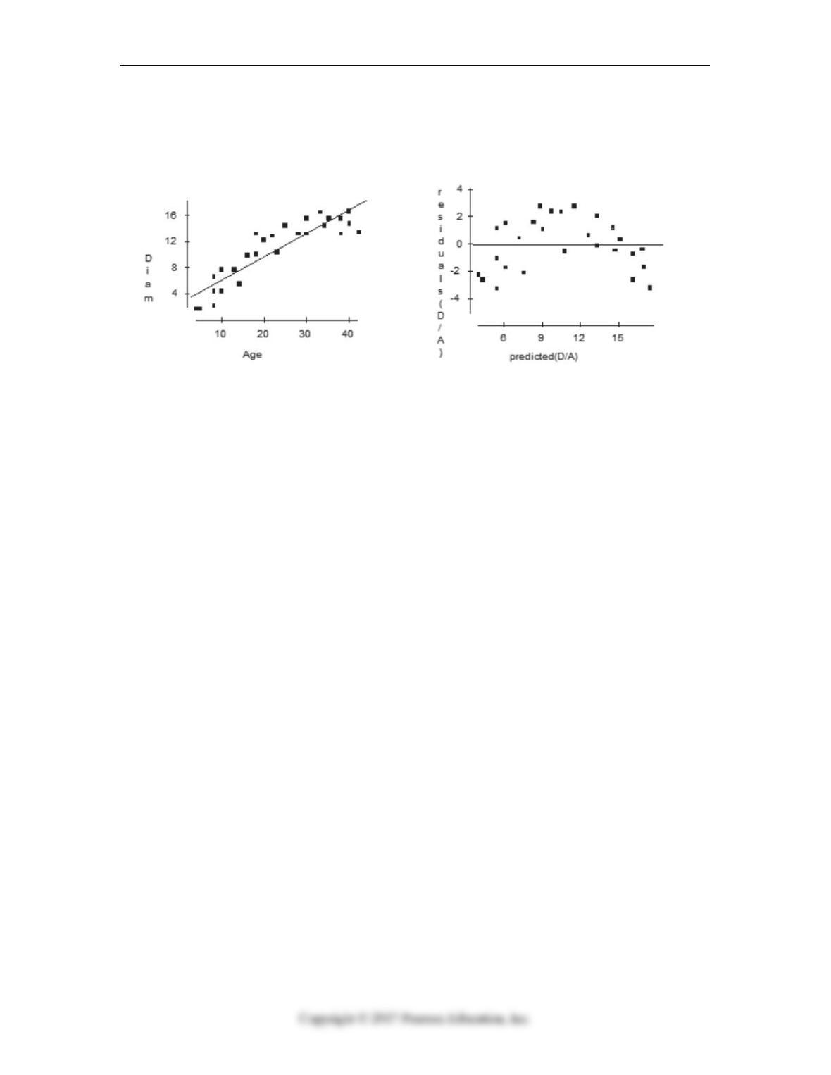
15. A linear model is fit to estimate the diameter of maple trees based on age. According
to the scatterplot and residual plots shown below, which of the following is true?
A. Assuming the pattern continues into the future, if we use this model to predict the
diameter of a maple tree that is 50 years old it would be too low.
B. Assuming the pattern continues into the future, if we use this model to predict the
diameter of a maple tree that is 50 years old it would be too high.
C. Re-expressing these data by taking the logarithm of age would improve this
model.
D. Both A and B.
E. Both B and C.
Chapter 14: Identify leveraged and/or influential points and determine if they affect the
model.
16. Which statement about influential points is true?
A. Removal of an influential point changes the regression line.
B. A high leverage point is always influential.
C. Influential points have large residuals.
D. All outliers are influential.
E. None of these.
Chapter 14: Determine when linear models are appropriate and/or useful for predicting
y-values.
17. A farmer has increased his wheat production by about the same amount each year.
His most useful predictive model is most probably
A. exponential.
B. linear.
C. logarithmic.
D. power.
E. quadratic.

Test A IVA-9
Chapter 15: Conduct inference on a multiple regression model.
18. The results of a multiple regression model to predict the job performance of new hires
based on age, GPA and gender (female = 1 and male = 0) resulted in an F-statistic of
30.23 and associated p-value of 0.000, we can conclude at α = .05 that
A. the regression equation is not significant.
B. all independent variables in the model are significant.
C. the regression equation is significant.
D. none of the independent variables in the model are significant.
E. both B and C.
Chapter 15: Determine, interpret, and apply multiple regression models.
19. According to the multiple regression model to predict the job performance of new
hires based on age, GPA and gender (female = 1 and male = 0) shown below, how
much of the variability in Job Performance is explained by the model?
The regression equation is
Job Performance = – 60.8 + 4.80 Age + 1.44 GPA + 9.06 Gender
Predictor Coef SE Coef T P
Constant -60.76 22.49 -2.70 0.012
Age 4.802 1.177 4.08 0.000
GPA 1.443 2.379 0.61 0.549
Gender 9.060 2.314 3.92 0.001
S = 5.56691 R-Sq = 77.7%
A. 30.33 %
B. 77.7 %
C. 5.56 %
D. 60.76 %
E. Cannot be determined.

IVA-10 Part IV: Models for Decision Making
Chapter 15: Determine, interpret, and apply multiple regression models.
20. The results of a multiple regression model to predict the job performance of new hires
based on age, GPA and gender (female = 1 and male = 0 are shown below. At α =
.05 we can conclude that
The regression equation is
Job Performance = – 60.8 + 4.80 Age + 1.44 GPA + 9.06 Gender
Predictor Coef SE Coef T P
Constant -60.76 22.49 -2.70 0.012
Age 4.802 1.177 4.08 0.000
GPA 1.443 2.379 0.61 0.549
Gender 9.060 2.314 3.92 0.001
S = 5.56691 R-Sq = 77.7%
A. Age is not a significant variable in predicting job performance.
B. GPA is a significant variable in predicting job performance.
C. The regression coefficient associated with GPA is significantly different from
zero.
D. Gender is a significant variable in predicting job performance.
E. The regression coefficient associated with Age is not significantly different from
zero.
Chapter 15: Understand and use dummy variables and/or interaction terms in regression
models.
21. The regression equation to predict the job performance of new hires based on age,
GPA and gender (female = 1 and male = 0) is Job Performance = -60.8 + 4.80
Age + 1.44 GPA + 9.06 Gender. Which of the following is the correct
interpretation for the regression coefficient of Gender?
A. The regression coefficient indicates that the job performance score for a female
will, on average, be 9.06 points higher than for males of the same age and GPA.
B. The regression coefficient indicates that the job performance score for a female
will, on average, be 9.06 points lower than for males of the same age and GPA.
C. The regression coefficient indicates that the job performance score for a female
will, on average, be 9.06 times higher than for males.
D. The regression coefficient indicates that the job performance score for a female
will, on average, be 9.06 times lower than for males.
E. The regression coefficient is not significantly different from zero.
Test A IVA-11
Business Statistics: Part IV: Models for Decision Making – Test A – Key