PTS: 1
6. Student enrollment at a university over the past six years is given below.
Year
Enrollment
(t)
(In 1,000s)
1
6.30
2
7.70
3
8.00
4
8.20
5
8.80
6
8.00
a.
Develop a linear trend expression for the above time series.
b.
Forecast enrollment for year 10.
b.
10,063
7. The following time series shows the sales of a clothing store over a 10-week period.
Week
Sales
($1,000s)
1
15
2
16
3
19
4
18
5
19
6
20
7
19
8
22
9
15
10
21
a.
Compute a 4-week moving average for the above time series.
b.
Compute the mean square error (MSE) for the 4-week moving average forecast.
c.
Use = 0.3 to compute the exponential smoothing values for the time series.
d.
Forecast sales for week 11.
17, 18, 19, 19, 20, 19
b.
7.67
15.00, 15.00, 15.30, 16.40, 16.89, 17.52, 18.26, 19.38, 18.07, 18.95
d.
$19,560
8. The following time series shows the number of units of a particular product sold over the past six
months.
Month
Units Sold
(Thousands)
1
8
2
3
3
4
4
5
5
12
6
10
a.
Compute a 3-month moving average (centered) for the above time series.
b.
Compute the mean square error (MSE) for the 3-month moving average.
c.
Use = 0.2 to compute the exponential smoothing values for the time series.
d.
Forecast the sales volume for month 7.
5, 4, 7
b.
MSE = 73/3 = 24.33
c.
8, 8, 7, 6.4, 6.12, 7.296
d.
9. The sales volumes of CMM, Inc., a computer firm, for the past 8 years is given below.
Year
Sales
(t)
(In Millions of Dollars)
1
2
2
3
3
5
4
4
5
6
6
8
7
9
8
9
a.
Develop a linear trend expression for the above time series.
b.
Forecast sales for period 9.
b.
$10,568,000
10. The sales records of a major auto manufacturer over the past ten years are shown below.
Year (t)
Number of Cars Sold
(In thousands of Units)
1
195
2
200
3
250
4
270
5
320
6
380
7
440
8
460
9
500
10
500
Develop a linear trend expression and project the sales (the number of cars sold) for time period t = 11
11. The following data show the quarterly sales of Amazing Graphics, Inc. for the years 6 through 8.
Year
Quarter
Sales
6
1
2.5
2
1.5
3
2.4
4
1.6
7
1
2.0
2
1.4
3
1.7
4
1.9
8
1
2.5
2
2.0
3
2.4
4
2.1
a.
Compute the four-quarter moving average values for the above time series.
b.
Compute the seasonal factors for the four quarters.
c.
Use the seasonal factors developed in Part b to adjust the forecast for the effect of season for
year 6.
Centered Moving Averages: 1.94; 1.87; 1.77; 1.72; 1.82; 1.96; 2.12; 2.26
b.
Seasonal Factors: 1.16; 0.85; 1.09; 0.92
c.
Deseasonalized Sales (Year 6): 2.16; 1.76; 2.20; 1.74
12. John has collected the following information on the amount of tips he has collected from parking cars
the last seven nights.
Day
Tips
1
18
2
22
3
17
4
18
5
28
6
20
7
12
a.
Compute the 3-day moving averages for the time series.
b.
Compute the mean square error for the forecasts.
c.
Compute the mean absolute deviation for the forecasts.
d.
Forecast John’s tips for day 7.
a.
19, 19, 21, 22, 20
b.
45.75
c.
5.25
d.
22
13. The following information has been collected on the sales of greeting cards for the past 6 weeks.
Week
Sales
1
105
2
90
3
95
4
110
5
105
6
100
a.
Produce exponential smoothing forecasts for the series using a smoothing constant of .2.
b.
Compute the mean square error for the forecasts produced with a smoothing constant of .2.
c.
What is the forecast of sales for week 7?
d.
Is a smoothing constant of .2 or .3 better for the sales data? Explain.
a.
105, 105, 102, 100.6, 102.48, 102.984
b.
75.523
c.
102.39
d.
0.2 is better since the MSE is smaller
14. Consider the following annual series on the number of people assisted by a county human resources
department.
Year
People (in 100s)
1
22
2
24
3
28
4
24
5
22
6
24
7
20
8
26
9
24
10
28
11
26
a.
Prepare 3-year moving average values to be used as forecasts for periods 4 through 11.
Calculate the mean squared error (MSE) measure of forecast accuracy for periods 4 through 11.
b.
Use a smoothing constant of .4 to compute exponential smoothing values to be used as
forecasts for periods 2 through 11. Calculate the MSE.
c.
Compare the results in Parts a and b.
a.
24.667, 25.333, 24.667, 23.333, 22, 23.333, 23.333, 26, MSE = 7.667
b.
22, 22.8, 24.88, 24.528, 23.5168, 23.71, 22.226, 23.7356, 23.8414, 25.505, MSE = 8.405
c.
The forecasts produced in Part a are better than those produced in Part b.
15. The temperature in Chicago has been recorded for the past seven days. You are given the information
below.
Day
Temperature
1
82
2
80
3
84
4
83
5
80
6
79
7
82
a.
Produce exponential smoothing forecasts for the series using a smoothing constant of .2.
b.
Compute the mean square error for the forecasts produced with a smoothing constant of .2.
c.
What is the forecasted temperature for day 8?
d.
Is a smoothing constant of .2 or .3 better for the temperature data? Explain.
a.
82, 81.6, 82.08, 82.264, 81.8112, 81.249
b.
4.033
c.
81.399
d.
A smoothing constant of 0.2 is better because the MSE is lower when 0.2 is used.
16. The yearly series below exhibits a long-term trend. Use the appropriate forecasting technique to
produce forecasts for years 11 and 12.
Year
Time Series Value
1
120
2
132
3
148
4
152
5
160
6
175
7
182
8
190
9
195
10
205
T = 115.2 + 9.218182t
17. The following time series gives the number of units sold during 5 years at a boat dealership.
Year
Quarter
Number of Units
1
1
300
2
240
3
240
4
290
2
1
350
2
300
3
280
4
320
3
1
410
2
400
3
390
4
410
4
1
490
2
450
3
440
4
510
5
1
540
2
530
3
520
4
540
a.
Find the four-quarter centered moving averages.
b.
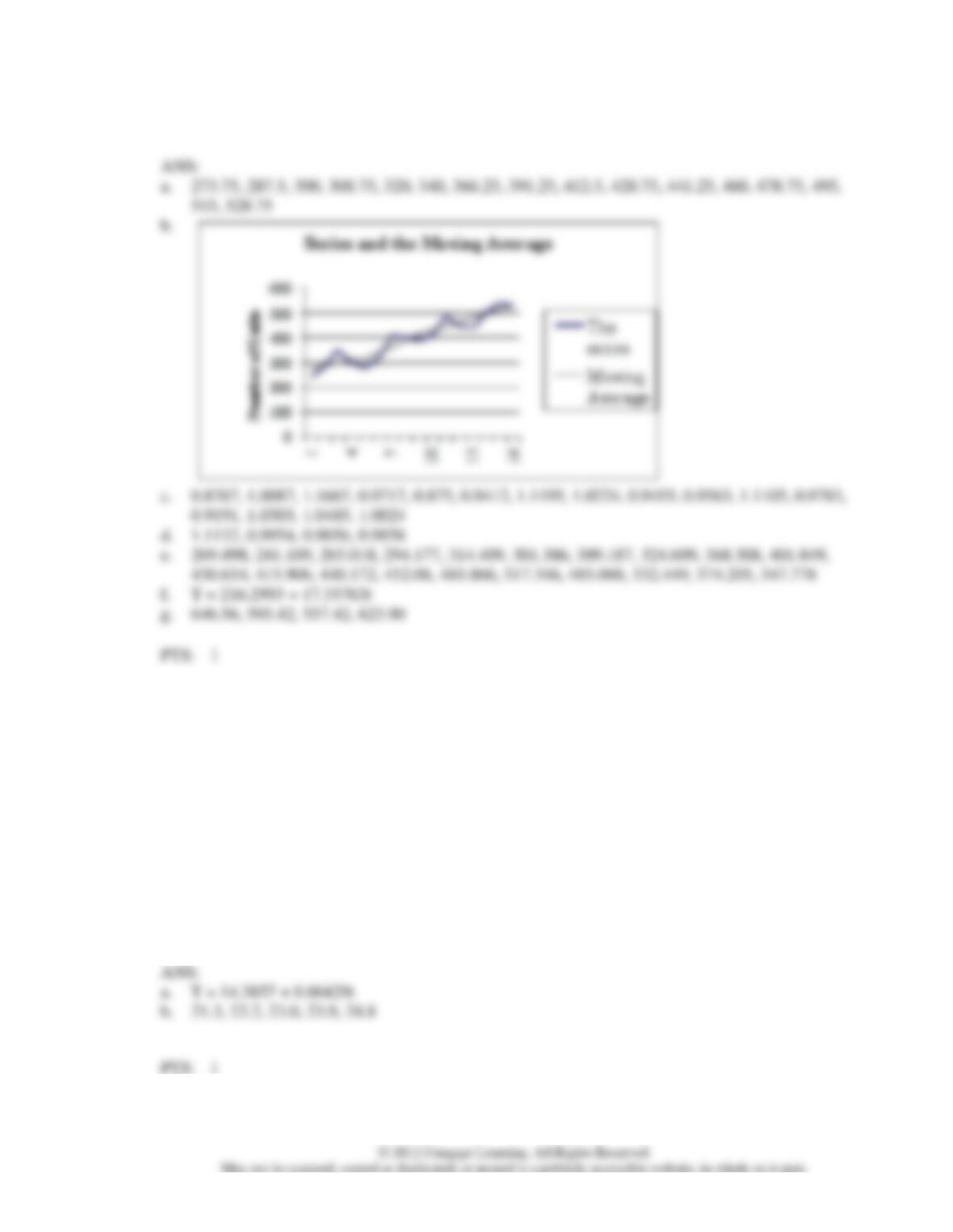
Plot the series and the moving averages on a graph.
c.
Compute the seasonal-irregular component.
d.
Compute the seasonal factors for all four quarters.
e.
Compute the deseasonalized time series for sales.
f.
Calculate the linear trend from the deseasonalized sales.
g.
Forecast the number of units sold in each quarter of year 6.
515, 528.75
d.
1.1132, 0.9954, 0.9056, 0.9858
430.654, 415.906, 440.172, 452.08, 485.866, 517.346, 485.088, 532.449, 574.205, 547.778
f.
T = 216.2993 + 17.35763t
g.
646.56, 595.42, 557.42, 623.90
18. Below you are given information on John’s income for the past 7 years.
Year
Income (In Thousands)
1
15.0
2
16.2
3
17.1
4
18.1
5
18.8
6
19.2
7
20.5
a.
Use regression analysis to obtain an expression for the linear trend component.
b.
Forecast John’s income for the next 5 years.
T = 14.3857 + 0.86429t
b.
21.3, 22.2, 23.0, 23.9, 24.8
19. You are given the following information on the quarterly profits for Ajax Corporation.
Year
Quarter
Quarterly Profits Yt
1
1
150
2
120
3
160
4
150
2
1
150
2
130
3
180
4
160
3
1
170
2
140
3
200
4
180
4
1
200
2
150
3
230
4
200
a.
Find the four-quarter centered moving averages.
b.
Compute the seasonal-irregular component.
c.
Compute the seasonal factors for all four quarters.
d.
Represent the deseasonalized series.
145, 146.25, 150, 153.75, 157.5, 161.25, 165, 170, 176.25, 181.25, 186.25, 192.5
b.
1.103, 1.026, 1, 0.846, 1.143, 0.992, 1.03, 0.824, 1.135, 0.993, 1.074, 0.779
c.
1.04, 0.82, 1.132, 1.008
20. Below you are given information on crime statistics for Middletown.
Year
Quarter
Number of Crimes Committed Yt
1
1
10
2
20
3
25
4
5
2
1
10
2
30
3
35
4
25
3
1
20
2
40
3
35
4
15
4
1
20
2
50
3
45
4
35
The seasonal factors for these data are
Quarter
Seasonal Factor St
1
.589
2
1.351
3
1.335
4
.726
a.
Deseasonalize the series.
b.
Obtain an estimate of the linear trend for this series.
c.
Use the seasonal and trend components to forecast the number of crimes for each quarter of
Year 5.
33.71, 48.21
b.
T = 13.5155 + 1.603765t
24.02, 57.26, 58.72, 33.1
21. Below you are given the seasonal factors and the estimated trend equation for a time series. These
values were computed on the basis of 5 years of quarterly data.
Quarter
Seasonal Factor St
1
1.2
2
.9
3
.8
4
1.1
T = 126.23 – 1.6t
Produce forecasts for all four quarters of year 6 by using the seasonal and trend components.
22. The following data show the quarterly sales of a major auto manufacturer (introduced in exercise 4) for
the years 8 through 10.
Year
Quarter
Sales
8
1
160
2
180
3
190
4
170
9
1
200
2
210
3
260
4
230
10
1
210
2
240
3
290
4
260
a.
Compute the four-quarter moving average values for the above time series.
b.
Compute the seasonal factors for the four quarters.
c.
Use the seasonal factors developed in Part b to adjust the forecast for the effect of season for
year 9.
180.00, 188.75, 201.25, 217.50, 226.25, 231.25, 238.75, 245.25
213.90, 215.38, 236.36, 243.39
23. Connie Harris, in charge of office supplies at First Capital Mortgage Corp., would like to predict the
quantity of paper used in the office photocopying machines per month. She believes that the number
of loans originated in a month influence the volume of photocopying performed. She has compiled
the following recent monthly data:
Number of Loans
Sheets of Photocopy
Originated in Month
Paper Used (000’s)
25
16
25
13
35
18
40
25
40
21
45
22
50
24
60
25
a. Develop the least-squares estimated regression equation that relates sheets of photocopy paper used
to loans originated.
b). Use the regression equation developed in part (a) to forecast the amount of paper used in a month
when 65 loan originations are expected.
24. The number of haircuts performed each day at KwikKuts in the last four weeks are listed below.
Week
Monday
Tuesday
Wednesday
Thursday
Friday
1
122
122
103
133
98
2
127
130
106
137
97
3
126
131
111
151
104
4
135
135
110
146
107
a. Plot the sales data. Do you see both trend and seasonality components in the data?
b. Forecast the number of haircuts to be performed in each workday of week 6.
25. Four months ago, the Bank Drug Company introduced Jeffrey William brand designer bandages.
Advertised using the slogan, “What the best dressed cuts are wearing”, weekly sales for this period (in
1000’s) have been as follows:
Week
Sales
Week
Sales
Week
Sales
1
12.8
7
20.6
12
23.8
2
14.6
8
18.5
13
25.1
3
15.2
9
19.9
14
24.7
4
16.1
10
23.6
15
26.5
5
15.8
11
24.2
16
28.9
6
17.2
a) Plot a graph of sales vs. weeks. Does linear trend appear reasonable?
b) Assuming linear trend, forecast sales for weeks 17, 18, 19, and 20.
26. Weekly sales of the Weber Dicamatic food processor for the past ten weeks have been:
Week
Sales
Week
Sales
1
980
6
990
2
1040
7
1030
3
1120
8
1260
4
1050
9
1240
5
960
10
1100
a. Determine, on the basis of minimizing the mean square error, whether a three period or four period
simple moving average model gives a better forecast for this problem.
b. For each model, forecast sales for week 11.
27. The number of new central air conditioning systems installed by CoolBreeze, Inc. in each of the last
nine years are listed below.
Year
Jobs
Year
Jobs
Year
Jobs
2002
353
2005
374
2008
399
2003
387
2006
396
2009
412
2004
342
2007
409
2010
408
Assuming a linear trend function, forecast the number of system installations CoolBreeze will perform
in 2011 using linear trend regression.
28. Delta Corp’s plant in Austin has been experiencing imbalances in its inventory of components used in
the production of a line of computer printers. Both stock shortages and overstock conditions are
occurring.
The production analysis group is studying the pattern of demand for component PS2400, a power
supply used in many of Delta’s products. The group believes that the most recent 12 weeks of
demand for the PS2400 is representative of the future weekly demand:
Week
Demand
(Units)
Week
Demand
(Units)
Week
Demand
(Units)
Week
Demand
(Units)
1
159
4
161
7
203
10
168
2
217
5
173
8
195
11
198
3
186
6
157
9
188
12
159
a. Use a four-week moving average to develop a forecast of the demand for the PS2400 component in
week 13.
b. Use a four-week weighted moving average with weights of .4 (for the most recent datum), .3, .2, and
.1 to forecast the demand for the PS2400 component in week 13.