
Name:
Class:
Date:
chapter 15
Indicate whether the statement is true or false.
1. RISKSIMTABLE is a function in @Risk for running several simulations simultaneously, one for each setting
of an input or decision variable.
a.
True
b.
False
2. A probability distribution is continuous if its possible values are essentially some continuum.
a.
True
b.
False
3. Sometimes it is convenient to treat a discrete probability distribution as continuous, and vice versa.
a.
True
b.
False
4. A correlation matrix must always be symmetric, so that the correlations above the diagonal are a mirror
image of those below it.
a.
True
b.
False
5. When we run simulation, the @Risk automatically keeps statistics such as averages and standard
deviations, and can also create graphs such as histograms based on the values generated in the output cells
in the simulation model.
a.
True
b.
False
6. A discrete distribution is useful for many situations, either when the uncertain quantity is not really
continuous (the number of televisions demanded, for example) or when you want a discrete approximation to a
continuous variable.
a.
True
b.
False
7. Analysts often plan a simulation so that the confidence interval for the mean of some important output will be
sufficiently narrow. The reasoning is that narrow confidence intervals imply more precision about the estimated
mean of the output variable.
a.
True
b.
False
8. It is common in computer simulations to estimate the mean of some distribution by the average of the
simulated observations. The usual practice is then to accompany this estimate with a confidence interval,
which indicates the accuracy of the estimate.
a.
True
b.
False
9. Spreadsheet simulation modeling is quite similar to the other modeling applications in that it begins with
input variables and then relates these with appropriate Excel formulas to produce output variables of interest.
a.
True
b.
False

Name:
Class:
Date:
chapter 15
10. If we want to model a random stock price, we should do so with an unbounded symmetric probability
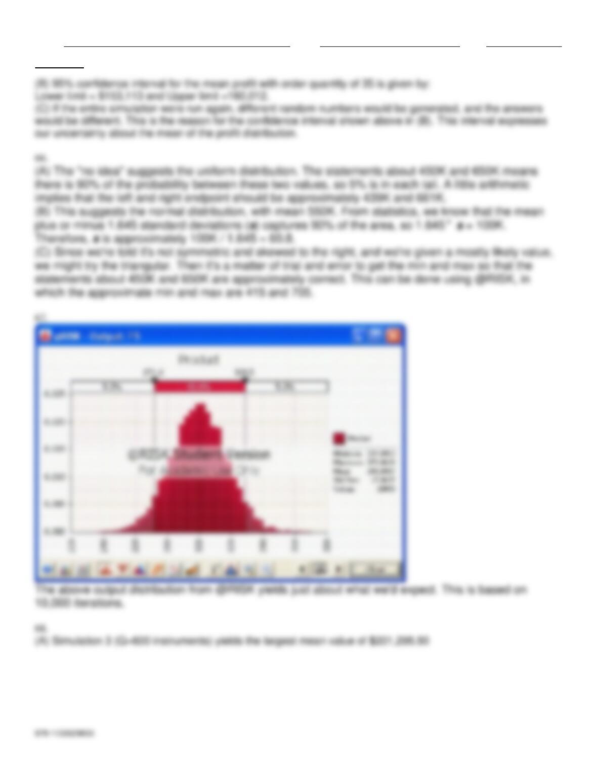
distribution.
a.
True
b.
False
11. A probability distribution is bounded if there are values A and B such that only one possible value can be
less than A or greater than B.
a.
True
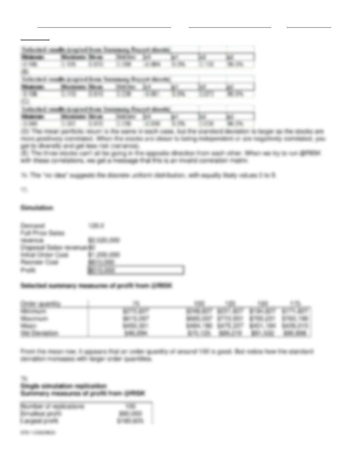
b.
False
12. A correlation matrix must always have 1’s along its diagonal (because a variable is always perfectly
correlated with itself) and the correlations between variables elsewhere.
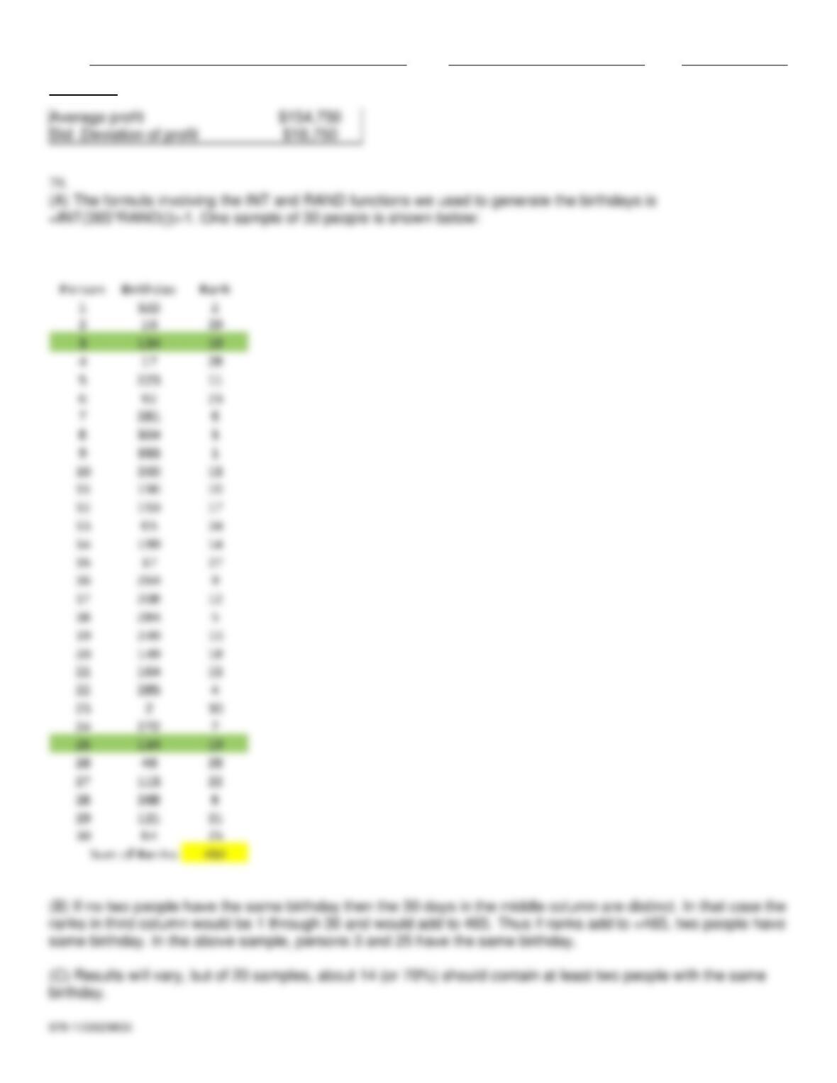
a.
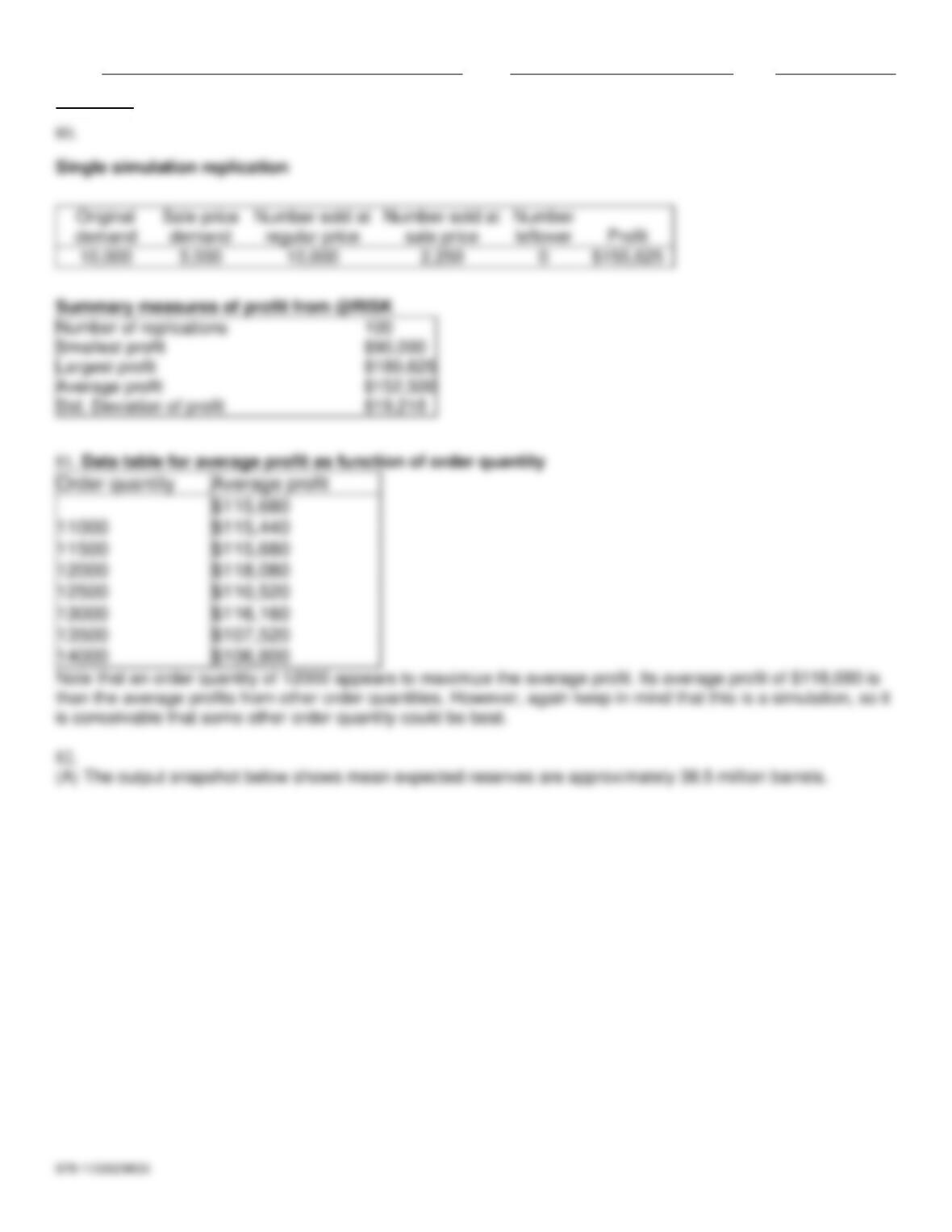
True
b.
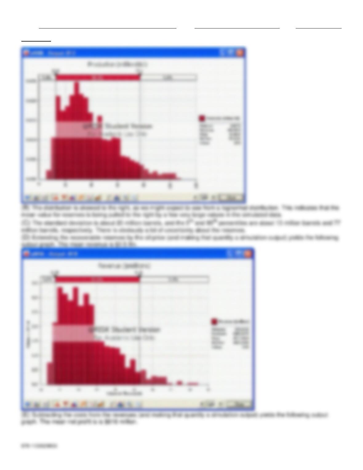
False
13. The triangular distribution is sometimes used in simulation models because it is more flexible and intuitive
than the normal distribution.
a.
True
b.
False
14. When we maximize or minimize the value of a decision variable by running several simulations
simultaneously, we have found an optimal solution to the problem and attitude toward risk becomes irrelevant.
a.
True
b.
False
15. The “random” numbers generated by the RAND function (or by any other package’s random number
generator) are not really random.
a.
True
b.
False
16. The normal distribution is often used in simulation models because it is the most common distribution in
statistics and it does not allow negative values.
a.
True
b.
False
17. The binomial distribution can be well approximated by the normal distribution when the number of trials n is
sufficiently small and the probability of success p is not too close to 0 or 1.
a.
True
b.
False
18. One of the primary advantages of simulation models that they enable managers to answer what-if
questions about changes in systems without actually changing the systems themselves.
a.
True
b.
False
19. Excel’s built-in functions, along with the RAND function, can be used to generate random numbers from
many different types of probability distributions.

Name:
Class:
Date:
chapter 15
a.
True
b.
False
20. Data tables in spreadsheet simulations are useful for taking a “prototype” simulation and replicating its key
results a desired number of times.
a.
True
b.
False
21. The binomial distribution is a discrete distribution that is applied to situations where n independent and
identical “trials” occur, with each trial resulting in a “success” or “failure,” and we want to generate the random
number of successes in the n trials.
a.
True
b.
False
22. The Excel RAND() function generates random numbers from a Normal(0,1) distribution.
a.
True
b.
False
23. We typically choose between a symmetric and skewed distribution on the basis of practical modeling
issues.
a.
True
b.
False
24. @Risk introduces uncertainty explicitly into a spreadsheet model by allowing several inputs to have
probability distributions and then enabling the simulation of random values from these inputs.
a.
True
b.
False
25. Correlation between two random input variables might not change the mean of an output, but it can
definitely affect the variability and shape of an output disbribution.
a.
True
b.
False
26. The uniform distribution is bounded by a minimum and a maximum, and all values between these two
extremes are equally likely.
a.
True
b.
False
27. The three parameters required to specify a triangular distribution are the minimum, mean and maximum.
a.
True
b.
False
28. Different random numbers generated by the computer are probabilistically dependent. This implies that
when we generate a random number in a particular cell, it has some effect on the values of any other random
numbers generated in the spreadsheet.
a.
True
b.
False

Name:
Class:
Date:
chapter 15
29. When you try to find the most appropriate input probability distribution in a simulation model, you first have
to choose the most appropriate family, and then you have to select the most appropriate member of that family
a.
True
b.
False
30. It is usually not too difficult to predict the shape of the output distribution from the shape(s) of the input
distribution(s).
a.
True
b.
False
31. A primary difference between standard spreadsheet models and simulation models is that at least one of
the input variable cells in a simulation model contains random numbers.
a.
True
b.
False
32. A common guideline in constructing confidence intervals for the mean is to place upper and lower bounds
one standard error on either side of the average to obtain an approximate 95% confidence interval.
a.
True
b.
False
33. The flaw of averages is the reason deterministic models can be very misleading.
a.
True
b.
False
Indicate the answer choice that best completes the statement or answers the question.
34. When n is reasonably large and p isn’t too close to 0 or 1, the binomial distribution can be well
approximated by which of the following distributions?
a.
Uniform distribution
b.
Normal distribution
c.
Triangular distribution
d.
None of these options
35. Which of the following statements are true?
a.
The @RISK contains a number of functions such as RISKNORMAL and RISKDISCRETE that make
it easy to generate observations from the most important probability distributions.
b.
You can specify any cell or range of cells in your simulation model as output cells.
When you run the simulation, @RISK automatically keeps summary measures (averages, standard
deviation, percentiles, and others) from the values generated in these output cells across the
replications.
c.
@RISK has a special function, RISKSIMTABLE, which allows you to run the same simulation
several times, using a different value of some key input variable each time.
d.
All of these options.
36. We can think of the uniform distribution as:
a.
the “I have no idea” distribution.
b.
a skewed distribution.

Name:
Class:
Date:
chapter 15
c.
only modeling positive values.
d.
nonnegative.
37. If a model contains uncertain outputs, it can be very misleading to build a deterministic model by using the
means of the inputs to predict an output. This is called the:
a.
Law of Large Numbers.
b.
Flaw of Averages
c.
Law of Inevitable Disappointment
d.
Central Limit Theorem
38. The RAND() function in excel models which of the following probability distributions:
a.
Normal(0,1)
b.
Uniform(0,1)
c.
Normal(-1,1)
d.
Uniform(-1,1).
39. The deterministic (non-simulation) approach, using best guesses for the uncertain inputs, is:
a.
better to use in complicated real world applications.
b.
a good estimate of what the answer will be using a simulation approach.
c.
generally not the appropriate model.
d.
the preferred approach when there is correlation between input variables.
40. A continuous probability distribution is characterized by a:
a.
mean and a standard deviation.
b.
mean and a variance.
c.
density function.
d.
histogram
41. Some important characteristics of probability distributions in general include the following distinctions:
a.
Discrete versus continuous
b.
Symmetric versus skewed
c.
Bounded versus unbounded
d.
Positive (or nonnegative) versus unrestricted
e.
All of these options
42. Which of the following statements is true regarding the Triangular distribution?
a.
It is a discrete distribution with a minimum, maximum and most likely value
b.
It is more flexible and intuitive than the normal distribution
c.
It is a symmetric distribution
d.
All of these options
43. If we want to model the monthly return on a stock, we might choose
a.
symmetric distribution around 0
b.
positively skewed distribution
c.
negatively skewed distribution

Name:
Class:
Date:
chapter 15
d.
All of these options
44. Which of the following statements is true regarding the Normal distribution?
a.
It is always the appropriate distribution in simulation modeling
b.
It does not permit negative values
c.
There is a 95% chance that values will be within ± 2 standard deviations of the mean
d.
All of these options
45. Many companies have used simulation to determine which of several possible investment projects they
should choose. This is often referred to as
a.
risk analysis
b.
@RISK investment
c.
unbounded risk
d.
None of the above
46. Simulation models are particularly useful for:
a.
forecasting.
b.
obtaining deterministic outputs.
c.
evaluating constraints.
d.
asking what-if questions.
47. Which of the following statements are false?
a.
A probability distribution is discrete if it has a finite number of possible values.
b.
A probability distribution is continuous if its possible values are essentially some continuum.
c.
An example of a discrete probability distribution is the amount of rain that falls during the month of
June in Michigan.
d.
None of these options
48. Which of the following statements are true?
a.
A probability distribution is symmetric (around some point) if the distribution to the left of the point is
a mirror image of the distribution to the right of the point.
b.
We say a distribution is skewed to the right (or positively skewed) if the “longer tail” is the right tail.
c.
We say a distribution is skewed to the left (or negatively skewed) if the “longer tail” is the left tail.
d.
All of the above
49. Which of the following statements are false regarding the numbers generated by the RAND function in
Excel?
a.
The numbers are random between 0 and 1
b.
The numbers are probabilistically dependent
c.
The numbers are probabilistically independent
d.
The numbers are uniformly distributed between 0 and 1
50. Which of the following statements is correct regarding the graph of a discrete probability distribution?
a.
It is a series of spikes.
b.
The height of each spike is the probability of the corresponding value.

Name:
Class:
Date:
chapter 15
c.
There is an empty space between adjacent spikes.
d.
All of these options
51. Which of the following statements is (are) false regarding the numbers generated by the RAND function in
Excel?
a.
Approximately 10% of the numbers will be between 0.0 and 1.0
b.
Approximately 20% of the numbers will be between 0.50 and 0.70
c.
Approximately 40% of the numbers will be between 0.20 and 0.60
d.
Approximately 60% of the numbers will be between 0.15 and 0.75
e.
All of these options are false
52. Suppose you run a simulation model several times with different order quantities. What can we infer about
the quantity that maximizes the output, the company’s profit?
a.
This quantity is the optimal order quantity.
b.
This quantity might be the optimal order quantity, but we also need to consider the company’s
attitude toward risk.
c.
This is not necessarily the optimal order quantity, because it may have produced the largest profit by
luck.
d.
We can’t infer anything.
53. We sometimes use discrete distributions in place of continuous distributions:
a.
because they are more accurate.
b.
because they are more simple.
c.
when we don’t know the mean and variance of the distribution.
d.
when we need to generate a histogram
54. If we want to model the time it takes to serve a customer at a bank, we will probably choose
a.
symmetric distribution
b.
positively skewed distribution
c.
negatively skewed distribution
d.
All of these options
55. A probability distribution is bounded if there are values A and B such that:
a.
A and B represent the 95% confidence interval
b.
A and B are the mean and standard deviation, respectively.
c.
A and B are the mean and variance, respectively.
d.
no value can be less than A or greater than B.
56. It is simple to generate a uniformly distributed random number with a minimum and maximum other than 0
and 1. For example, the formula =150+100 RAND() generates a number uniformly distributed between
a.
100 and 150
b.
150 and 250
c.
50 and 100
d.
50 and 250
57. One important special use of bounded distributions is when the only possible values are:

Name:
Class:
Date:
chapter 15
a.
less than zero.
b.
uniformly distributed around the mean.
c.
skewed to the right.
d.
nonnegative.
58. Each different set of values obtained for the uncertain quantities in a simulation model can considered to
be:
a.
the mean of the probability distribution.
b.
a scenario.
c.
a best guess.
d.
all of these options.
59. Which of the following statements are false regarding the graph of a continuous probability distribution?
a.
It is characterized by a density function, a smooth curve.
b.
It is a series of spikes
c.
The height of the density curve above any point is not actually a probability—that is, it is not
necessarily between 0 and 1.
d.
Heights above the density function indicate relative likelihoods but are not necessarily values
between 0 and 1.
60. In order to generate random numbers in Excel from a discrete distribution with a finite number of possible
values and corresponding probabilities, we can use
a.
only the RAND function
b.
only the VLOOKUP function
c.
only the VLOOKDOWN function
d.
the RAND function along with a VLOOKUP function
61. Which of the following statements is true regarding a simulation model?
a.
It explicitly models decision-making under uncertainty
b.
It explicitly incorporates uncertainty in one or more input variables
c.
It provides probability distributions for all outputs, rather than expected values
d.
All of these options
62. The “building blocks” of all spreadsheet simulation models are:
a.
deterministic inputs
b.
random numbers between 0 and 1
c.
decision variables
d.
probability distributions
63. Assume that x is a random number between 0 and 1, and that the number of units expected to be sold is
uniformly distributed between 300 and 500. Then, sales are given by the expression
a.
300 + x
b.
500 – x
c.
300 + 200 x
d.
500 – 200 x

Name:
Class:
Date:
chapter 15
e.
300 + 500 x
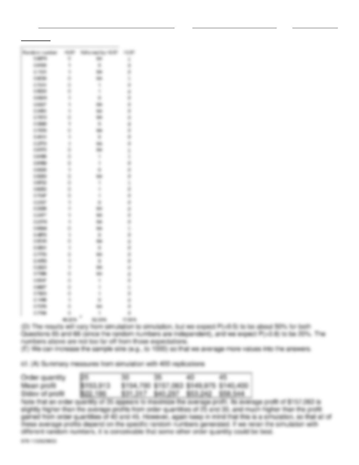
Generate a set of 40 random numbers in a column in an Excel spreadsheet by using RAND function. Fix the
set of random numbers by copying the column to another column and using the “Paste Special” command with
the “Values” option selected.
64. (A) What fraction of the random numbers are smaller than 0.5?
(B) What fraction of the time is a random number less than 0.5 followed by another random number less than
0.5?
(C) What fraction of the random numbers are larger than 0.8?
(D) What do you expect the answers to (A), (B) and (C) to be before simulating? Do the answers you provided
to those questions match your expectations? Explain why or why not.
(E) Suppose your answers to (A), (B) and (C) are not close to the expected answers. What can you do to
obtain answers from the simulation that are closer to the expected answers?
In August 2009, a car dealer is trying to determine how many 2010 cars to order. Each car ordered in August
2009 costs $16,000. The demand for the dealer’s 2010 models has the probability distribution shown in the
table below. Each car sells for $21,000. If the demand for 2010 cars exceeds the number of cars ordered in
August 2009, the dealer must reorder at a cost of $18,000 per car. Excess cars can be disposed of at $13,000
per car.
Cars demanded
Probability
25
0.25
30
0.20
35
0.15
40
0.20
45
0.20
65. (A) Use simulation to determine how many cars the dealer should order in August, 2009 to maximize his
expected profit.
(B) For the optimal order quantity, find a 95% confidence interval for the expected profit.
(C) Why is it important to develop the confidence interval in (B)?
A company is about to develop and then market a new product. It wants to build a simulation model for the
entire process, and one key uncertain input is the development cost. For each of the scenarios in the questions
below, choose an “appropriate” distribution, together with its parameters, and explain your choice.
66. (A) Company experts have no idea what the distribution of the development cost is. All they can state is
that “we are 90% sure it will be somewhere between $450,000 and $650,000.”
(B) Company experts can still make the same two statements as in (A), but now they can also state that “we
believe the distribution is symmetric and its most likely value is about $550,000.”
(C) Company experts can still make the same two statements as in (A), but now they can also state that “we
believe the distribution is skewed to the right, and its most likely value is about $500,000.”

Name:
Class:
Date:
chapter 15
67. If you add several normally distributed random numbers, the result is normally distributed, where the mean
of the sum is the sum of the individual means, and the variance of the sum is the sum of the individual
variances. This result is difficult to prove mathematically, but it is easy to demonstrate with simulation. To do
so, run a simulation where you add three normally distributed random numbers, each with mean 100 and
standard deviation 10. Your single output variable should be the sum of these three numbers. Verify with
@RISK that the distribution of this output is approximately normal with mean 300 and variance 300 (hence,
standard deviation = 17.32).
A fine arts institute is planning a summer camp where it will host young musicians from around the country one
year from now. Within the next two weeks, the organizers must decide how many violins to reserve with the
company that will provide instruments. On one hand, they do not want to reserve too few violins because if
they end up with more applicants than instruments available, they will have to turn applicants away. On the
other hand, they do not want to reserve too many violins because they pay a non-refundable cost of $500 for
each violin reserved. Based on historical data, the institute believes that the potential number of camp
participants has a normal distribution with mean 600 and standard deviation 100. Each potential camp
participant pays an $895 fee that covers all costs, including the instrument rental.
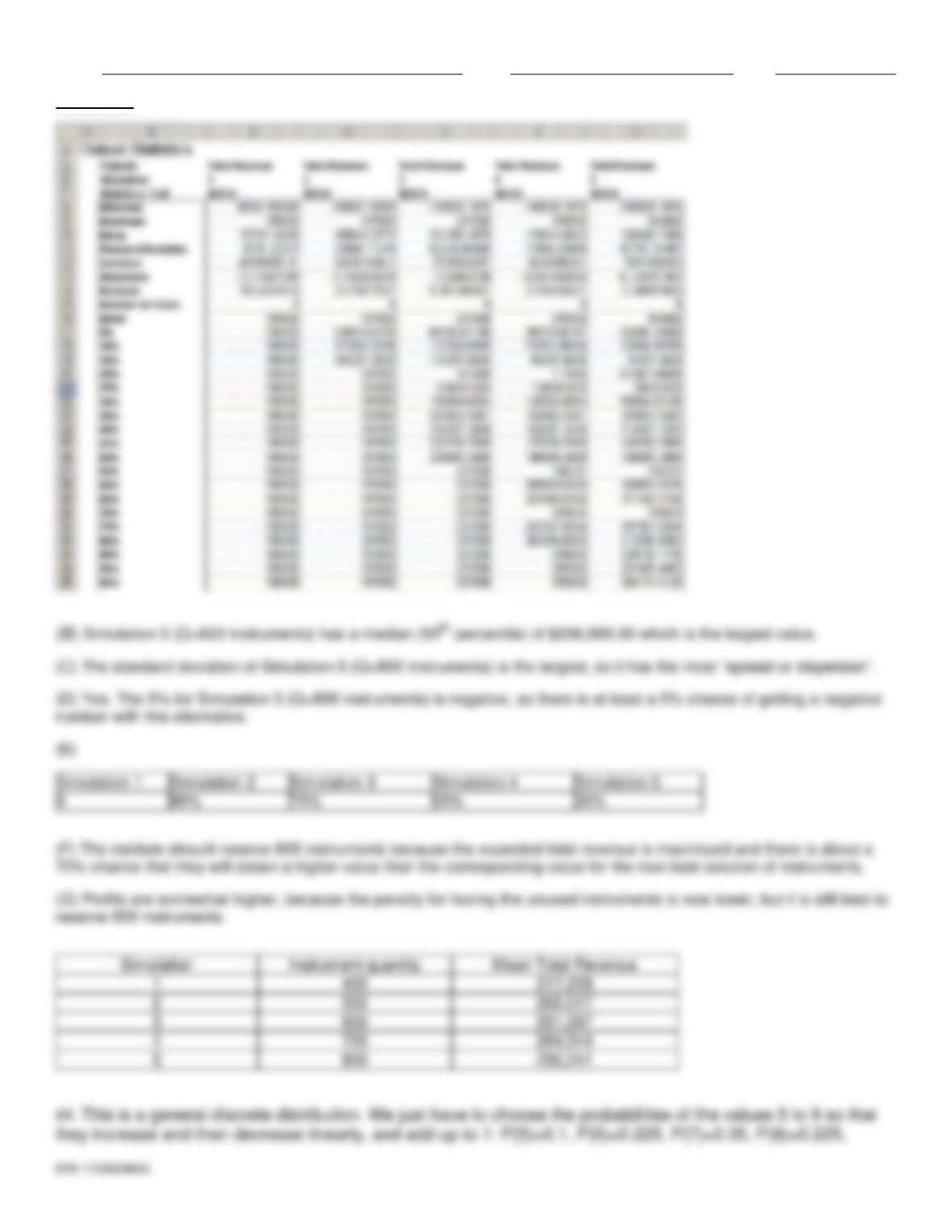
68. (A) Use a simulation model to help the institute decide how many violins they must reserve with the
instrument company. Consider five different possible reservation quantities: 400, 500, 600, 700, 800. Which of
these quantities yields the highest total revenue, net of instrument costs?
(B) Which simulation yields the largest median total revenue?
(C) Which simulation has the most risk as measured by spread or dispersion in the data? Please state clearly
what statistic you used to answer this question.
(D) Are there any simulations in which there is at least a 1 in 20 (i.e., 5%) chance of getting a negative total
revenue? Briefly explain in one sentence.
(E) For each simulation what is the probability of exceeding $175,000 in total revenue (approximate these
numbers as closely as possible from the data given in the above table). Please put your answer in the following
table:
Simulation 1
Simulation 2
Simulation 3
Simulation 4
Simulation 5
(F) Considering your answers for (A) through (E), please state how many instruments you think should be
reserved in advance and explain why.
(G) Suppose the institute is able to negotiate with the instrument company to reduce the cost for a violin from
$500 to $350. Re–run the simulation model using the same reservation quantities (but with $350 for the unused
instrument cost). Has the reservation quantity that yields the highest average revenue changed? If so, please
explain why this has occurred.
A company is about to develop and then market a new product. It wants to build a simulation model for the
entire process, and one key uncertain input is the development time, which is measured in an integer number
of months. For each of the scenarios in the questions below, choose an “appropriate” distribution, together with
its parameters, and explain your choice.
69. Company experts believe the development time will from 5 to 9 months. They believe the probabilities of
the extremes (5 and 9 months) are both 10%, and the probabilities will vary linearly from those endpoints to a
most likely value at 7 months.

Name:
Class:
Date:
chapter 15
A company produces six-packs of soda cans. Each can is supposed to contain at least 12 ounces of soda. If
the total weight in a six-pack is under 72 ounces, the company is fined $100 and receives no sales revenue for
the six-pack. Each six-pack sells for $3.00. It costs the company $0.02 per ounce of soda put in the cans. The
company can control the mean fill rate of its soda-filling machines. The amount put in each can by a machine is
normally distributed with standard deviation 0.10 ounce.
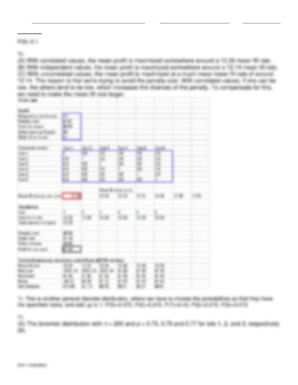
70. (A) Assume that the weight of each can in a six-pack has a 0,8 correlation with the weight of the other cans
in the six-pack. What mean fill quantity (within 0.05 ounce) maximizes expected profit per sic-pack?
(B) If the weights of the cans in the six-pack are probabilistically independent, what mean fill quantity (within
0.05 ounce) will maximize expected profit per six-pack?
(C) How can you explain the difference in the answers for (A) and (B)?
A company is about to develop and then market a new product. It wants to build a simulation model for the
entire process, and one key uncertain input is the development time, which is measured in an integer number
of months. For each of the scenarios in the questions below, choose an “appropriate” distribution, together with
its parameters, and explain your choice.
71. Company experts believe the development time will be from 5 to 9 months. They believe that 7 months is
twice as likely as either 6 months or 8 months and that either of these latter possibilities is three times as likely
as either 5 months or 9 months.
The College of Arts and Sciences at a Midwestern university currently has three parking lots, each containing
160 spaces. Two hundred faculty members have been assigned to each lot. On a peak day, the probability of a
lot 1 parking sticker holder showing up is 73%, a lot 2 parking sticker holders showing up is 75%, and a lot 3
parking sticker holder showing up is 77%.
72. (A) What are the appropriate probability distributions to model the number of faculty members showing up
in each lot?
(B) Given the current situation, estimate the probability that on a peak day, at least one faculty member with a
sticker will be unable to find a parking space. Assume that the number who shows up at each lot is
independent of the number who shows up at the other two lots.
(C) Suppose that faculty members are allowed to park in any lot. Does this help solve the problem? Why or
why not?
(D) Suppose that the numbers of faculty who show up at the three lots are correlated, with each correlation
equal to 0.80. Does your answer to (C) change? Why or why not?
Suppose that Mrs. Smart invested 25% of her portfolio in four different stocks. The mean and standard
deviation of the annual return on each stock are shown in the first table below. The correlations between the
annual returns on the four stocks are shown in the second table below.
Distributions of returns
Mean
Stdev
Stock 1
16%
21%
Stock 2
12%
13%
Stock 3
25%
38%
Stock 4
18%
20%
Correlation matrix

Name:
Class:
Date:
chapter 15
Stock 1
Stock 2
Stock 3
Stock 4
Stock 1
1.00
0.75
0.70
0.60
Stock 2
0.75
1.00
0.80
0.50
Stock 3
0.70
0.80
1.00
0.65
Stock 4
0.60
0.50
0.65
1.00
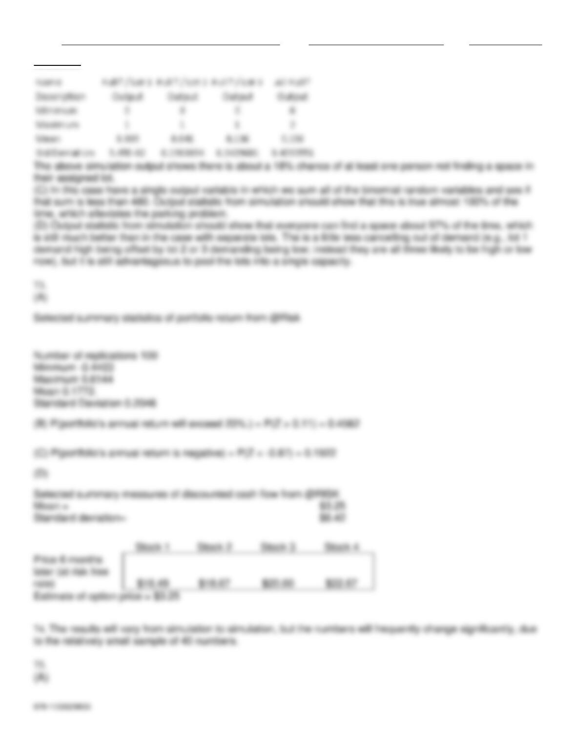
73. (A) Use @Risk with 100 replications, provide a summary statistics of portfolio return; namely, minimum,
maximum, mean, and standard deviation.
(B) Use your answers to (A) to estimate the probability that Mrs. Smart’s portfolio’s annual return will exceed
20%.
(C) Use your answers to (A) to estimate the probability that Mrs. Smart’s portfolio will lose money during the
course of a year.
(D) Suppose that the current price of each stock is as follows: stock 1: $16; stock 2: $18; stock 3: $20; and
stock 4: $22. Mrs. Smart has just bought an option involving these four stocks. If the price of stock 1, six
months from now are is $18 or more, the option enables Mrs. Smart to buy, if she desires, one share of each
stock for $20 six months from now. Otherwise the option is worthless. For example, if the stock prices six
months from now are: stock 1: $18; stock 2: $20; stock 3: $21; and stock 4: $24, then Mrs. Smart would
exercise her option to buy stocks 3 and 4 and receive (21- 20) + (24-20) = $5 in each cash flow. How much is
this option worth if the risk-free rate is 8%?
Generate a set of 40 random numbers in a column in an Excel spreadsheet by using RAND function. Fix the
set of random numbers by copying the column to another column and using the “Paste Special” command with
the “Values” option selected.
74. Obtain another set random numbers by pressing the F9 (recalculate) key. Do your results change
significantly? Do the changes match your expectations? Explain your answer.
Suppose you are going to invest equal amounts in three stocks. The annual return from each stock is normally
with mean 0.01 (1%) and standard deviation 0.06. The annual return on your portfolio, the output variable of
interest, is the average of the three stock returns. Run @RISK, using 1000 iterations, on each of the scenarios
described in the questions below, and report few results from the summary report sheets.
75. (A) The three stock returns are highly correlated. The correlation between each pair is 0.9
(B) The three stock returns are practically independent. The correlation between each pair is 0.1
(C) The first two stocks are moderately correlated. The correlation between their returns is 0.4. The third
stock’s return is negatively correlated with the other two. The correlation between its return and each of the first
two is -0.8.
(D) Compare the portfolio distributions from @RISK for the three scenarios in (A), (B) and (C). What do you
conclude?
(E) You might think of a fourth scenario, where the correlation between each pair of returns is a large negative
number such as -0.80. But explain intuitively why this makes no sense. Try running a simulation with these
negative correlations to see what happens.
A company is about to develop and then market a new product. It wants to build a simulation model for the
entire process, and one key uncertain input is the development time, which is measured in an integer number
of months. For each of the scenarios in the questions below, choose an “appropriate” distribution, together with
its parameters, and explain your choice.

Name:
Class:
Date:
chapter 15
76. Company experts believe the development time will be from 5 to 9 months, but they have absolutely no
idea which of these will result.
In August 2009, a car dealer is trying to determine how many 2010 cars to order. Each car ordered in August
2009 costs $16,000. The demand for the dealer’s 2010 models has the probability distribution shown in the
table below. Each car sells for $21,000. If the demand for 2010 cars exceeds the number of cars ordered in
August 2009, the dealer must reorder at a cost of $18,000 per car. Excess cars can be disposed of at $13,000
per car.
Cars demanded
Probability
25
0.25
30
0.20
35
0.15
40
0.20
45
0.20
77. Suppose that the demand for cars is normally distributed with mean of 120 and standard deviation of 20.
Use @Risk simulation add-in to determine the “best” order quantity; that is, the one that has the largest
expected profit. Using the statistics and/or graphs from @Risk, discuss whether this order quantity would not
be considered the “best” by the car dealer.
After Michigan State University reached the final four in the 2000 NCAA Basketball Tournament, a sweatshirt
supplier in Lansing is trying to decide how many sweatshirts to print for the upcoming championships. The final
four teams (Michigan State, Florida, Wisconsin, and North Carolina) have emerged from the quarterfinal round,
and there is a week left until the semifinals, which are then followed in a couple of days by the finals. Each
sweatshirt costs $12 to produce and sells for $24. However, in three weeks, any leftover sweatshirts will be put
on sale for half price, $12. The supplier assumes that the demand (in thousands) for his sweatshirts during the
next three weeks, when interest is at its highest, follows the probability distribution shown in the table below.
The residual demand, after the sweatshirts have been put on sale, also has the probability distribution shown
in the table below. The supplier realizes that every sweatshirt sold, even at the sale price, yields a profit.
However, he also realizes that any sweatshirts produced but not sold must be thrown away, resulting in a $12
loss per sweatshirt.
Demand distribution at regular price Demand distribution at reduced price
Demand
Probability
Demand
Probability
7
0.05
2
0.20
8
0.10
3
0.30
9
0.25
4
0.20
10
0.30
5
0.15
11
0.20
6
0.10
12
0.10
7
0.05
78. Use @Risk simulation add–in to analyze the sweatshirt sales. Do this for the discrete distributions given in
the problem.
It is surprising (but true) that if 23 randomly selected people are in the same room, there is about a 50%
chance that at least two people will have the same birthday. Suppose you want to estimate the probability that
if 30 people are in the same room, at least two of them will have the same birthday. You can proceed as
follows:
79. (A) Generate the “birthdays” of 30 different people, assuming that each person has a 1/365 chance of
having a given birthday (call the days of the year 1, 2, 3, ……..,365). You can use a formula involving the

Name:
Class:
Date:
chapter 15
DISCRETE and RAND functions to generate birthdays.
(B) Once you have generated 30 people’s birthdays, you can tell whether at least two people have the same
birthday using Excel’s RANK function (i.e., in the case of a tie, two numbers are given the same rank). Do you
see any people with the same birthday in your sample?
(C) Obtain at least 20 samples of the 30 person group using the F9 key. What do you estimate the probability
of finding two people with the same birthday in a sample of 30 people to be?
After Michigan State University reached the final four in the 2000 NCAA Basketball Tournament, a sweatshirt
supplier in Lansing is trying to decide how many sweatshirts to print for the upcoming championships. The final
four teams (Michigan State, Florida, Wisconsin, and North Carolina) have emerged from the quarterfinal round,
and there is a week left until the semifinals, which are then followed in a couple of days by the finals. Each
sweatshirt costs $12 to produce and sells for $24. However, in three weeks, any leftover sweatshirts will be put
on sale for half price, $12. The supplier assumes that the demand (in thousands) for his sweatshirts during the
next three weeks, when interest is at its highest, follows the probability distribution shown in the table below.
The residual demand, after the sweatshirts have been put on sale, also has the probability distribution shown
in the table below. The supplier realizes that every sweatshirt sold, even at the sale price, yields a profit.
However, he also realizes that any sweatshirts produced but not sold must be thrown away, resulting in a $12
loss per sweatshirt.
Demand distribution at regular price Demand distribution at reduced price
Demand
Probability
Demand
Probability
7
0.05
2
0.20
8
0.10
3
0.30
9
0.25
4
0.20
10
0.30
5
0.15
11
0.20
6
0.10
12
0.10
7
0.05
80. Use @Risk simulation add–in to analyze the sweatshirt sales. Do this for normal distributions, where we
assume that the regular demand is normally distributed with mean 10,000 and standard deviation 1500, and
that the demand at the reduced price is normally distributed with mean 5,000 and standard deviation 1500.
81. Use simulation to analyze the supplier’s problem. Determine how many sweatshirts he should produce to
maximize the expected profit.
An oil company is trying to determine the amount of oil that it can expect to recover from an oil field. The
unknowns are: the area of the field (in acres), the thickness of the oil-sand layer, and the primary recovery
factor (in barrels per acre per foot of thickness). Based on geological information, the following probability
distributions have been estimated.
Estimate of Productive Area
Acres Probability
9,000 0.05
10,000 0.10
11,000 0.15
12,000 0.35
13,000 0.25
14,000 0.10
Estimate of Pay Thickness

Name:
Class:
Date:
chapter 15
Smallest Value: 15 ft
Most Likely Value: 50 ft
Largest Value: 120 ft
Estimate of Primary Recovery
Minimum Value: 20 bbl./acre-ft
Maximum Value: 90 bbl./acre-ft
The amount of reserves that can be produced is then the product of the area, thickness, and recovery factor:
Number of barrels = Productive Area x Pay Thickness x Primary Recovery Factor
82. (A) Use @RISK distributions to generate the three random variables and derive a distribution for the
amount of reserves. What is the amount we can expect to recover from this field?
(B) The production output is a product of three very different types of input distributions. What does the output
distribution look like? What are the implications of the shape of this distribution?
(C) What is the standard deviation of the recoverable reserves? What are the 5th and 95th percentiles of this
distribution? What does this imply about the uncertainty in estimating the amount of recoverable reserves?
(D) Suppose you think oil price is normally distributed with a mean of $65 per barrel and a standard deviation
of $10. How much revenue do you expect the field produce (ignore discounting)?
(E) Finally, your engineer is uncertain about costs to drill wells to develop the field, but she thinks the most
likely cost will be $1.7Bn, although it could be as much as $3Bn or as little as $1Bn. What is your expected
profit from the field?
(F) What is the chance that you will lose money? Is this a risky venture?
Name:
Class:
Date:
chapter 15
Answer Key
Name:
Class:
Date:
chapter 15
Name:
Class:
Date:
chapter 15
Name:
Class:
Date:
chapter 15
Name:
Class:
Date:
chapter 15
Name:
Class:
Date:
chapter 15
Simulation 1
Simulation 2
Simulation 3
Simulation 4
Simulation 5
0
Name:
Class:
Date:
chapter 15
Name:
Class:
Date:
chapter 15
Name:
Class:
Date:
chapter 15
Name:
Class:
Date:
chapter 15
Name:
Class:
Date:
chapter 15
Name:
Class:
Date:
chapter 15
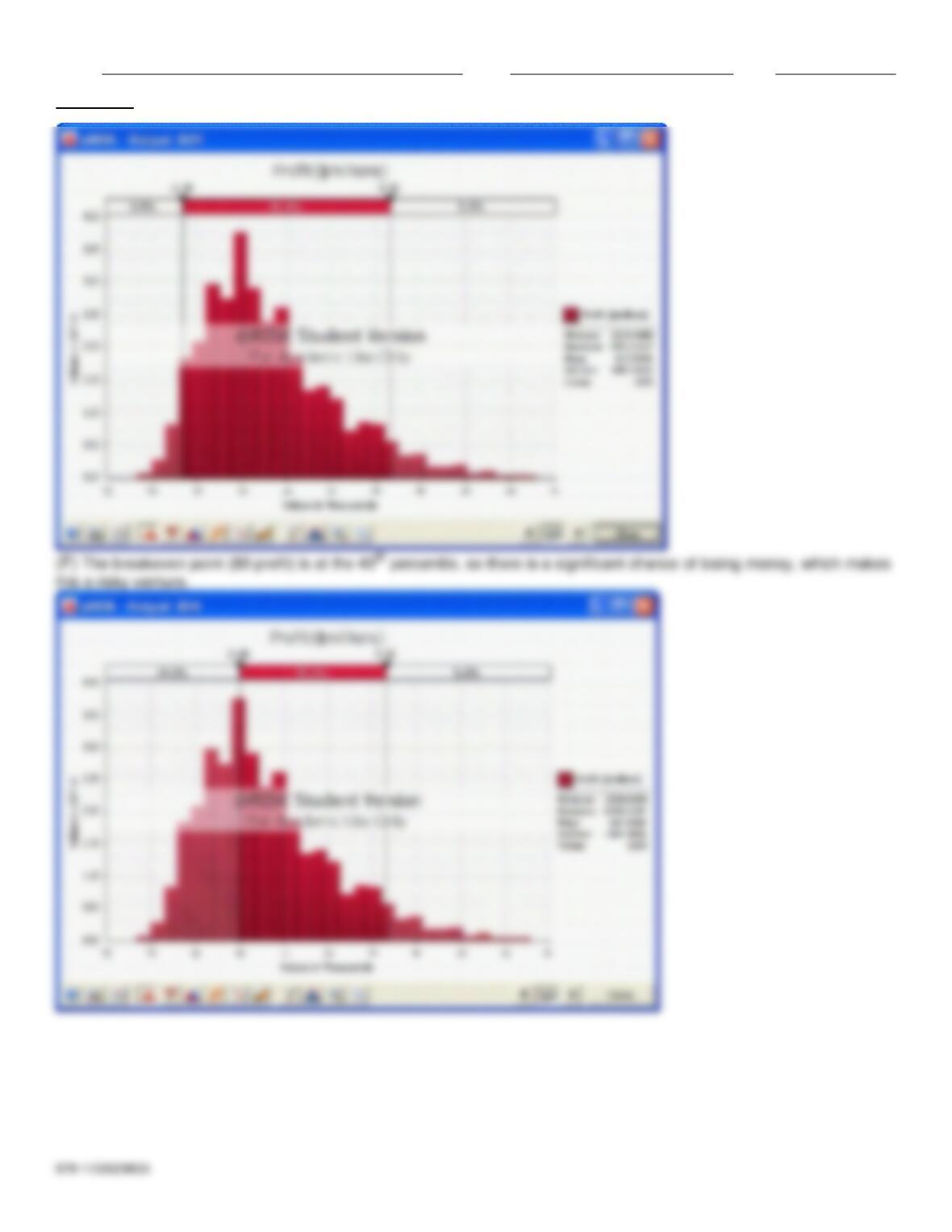
graph. The mean net profit is is $618 million.
Name:
Class:
Date:
chapter 15